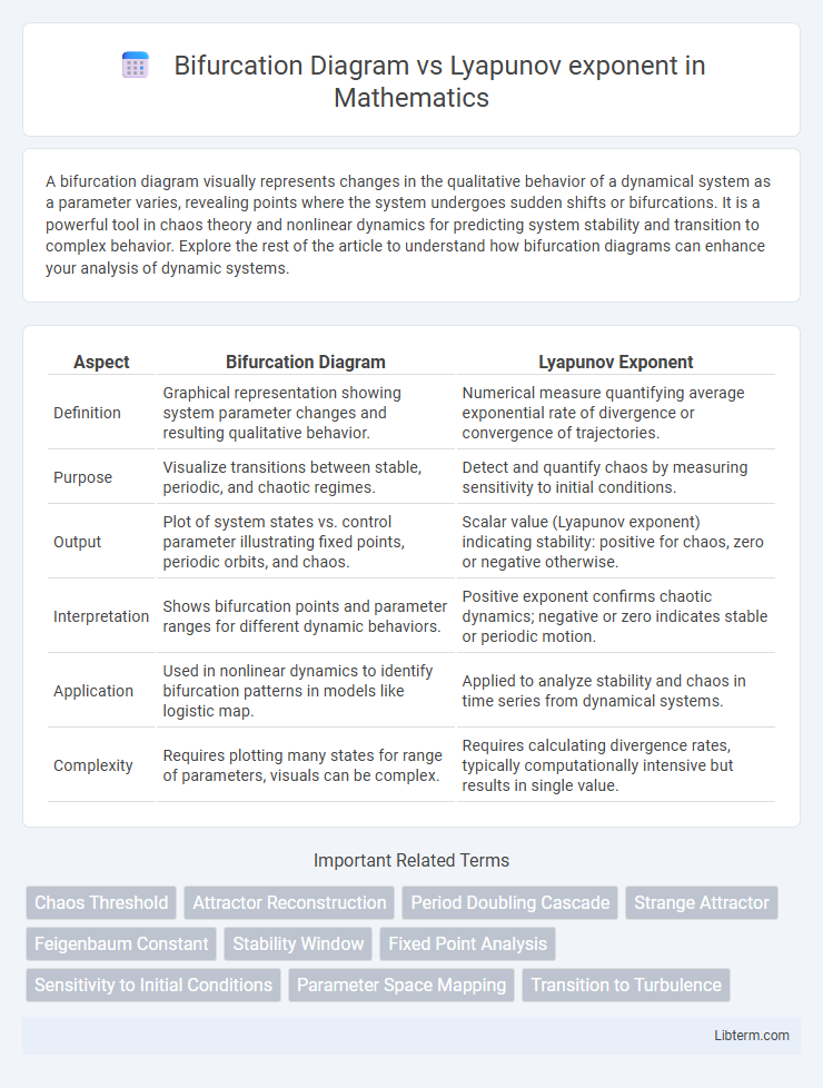
A bifurcation diagram visually represents changes in the qualitative behavior of a dynamical system as a parameter varies, revealing points where the system undergoes sudden shifts or bifurcations. It is a powerful tool in chaos theory and nonlinear dynamics for predicting system stability and transition to complex behavior. Explore the rest of the article to understand how bifurcation diagrams can enhance your analysis of dynamic systems.
Table of Comparison
| Aspect | Bifurcation Diagram | Lyapunov Exponent |
|---|---|---|
| Definition | Graphical representation showing system parameter changes and resulting qualitative behavior. | Numerical measure quantifying average exponential rate of divergence or convergence of trajectories. |
| Purpose | Visualize transitions between stable, periodic, and chaotic regimes. | Detect and quantify chaos by measuring sensitivity to initial conditions. |
| Output | Plot of system states vs. control parameter illustrating fixed points, periodic orbits, and chaos. | Scalar value (Lyapunov exponent) indicating stability: positive for chaos, zero or negative otherwise. |
| Interpretation | Shows bifurcation points and parameter ranges for different dynamic behaviors. | Positive exponent confirms chaotic dynamics; negative or zero indicates stable or periodic motion. |
| Application | Used in nonlinear dynamics to identify bifurcation patterns in models like logistic map. | Applied to analyze stability and chaos in time series from dynamical systems. |
| Complexity | Requires plotting many states for range of parameters, visuals can be complex. | Requires calculating divergence rates, typically computationally intensive but results in single value. |
Introduction to Nonlinear Dynamics
Bifurcation diagrams and Lyapunov exponents are fundamental tools in nonlinear dynamics used to analyze system behavior and stability. The bifurcation diagram visually represents changes in system states as parameters vary, highlighting transitions such as period doubling and chaos onset. Lyapunov exponents quantify sensitivity to initial conditions, with positive values indicating chaotic dynamics, thereby complementing bifurcation analysis in understanding complex nonlinear systems.
What Is a Bifurcation Diagram?
A bifurcation diagram visualizes how the qualitative behavior of a dynamical system changes as a control parameter varies, showing transitions between stable states and chaotic regimes. It plots the possible long-term values (fixed points, periodic orbits) of the system against the parameter, revealing bifurcations where the system behavior splits or changes stability. This tool contrasts with the Lyapunov exponent, which quantifies the sensitivity to initial conditions, but the bifurcation diagram provides a more intuitive view of system dynamics and parameter-dependent transitions.
Understanding the Lyapunov Exponent
The Lyapunov exponent quantifies the rate of separation of infinitesimally close trajectories in a dynamical system, serving as a critical measure of chaos and system stability. Unlike the bifurcation diagram, which visually maps the qualitative changes in system behavior as a parameter varies, the Lyapunov exponent provides a precise numerical value indicating whether the system exhibits convergence (negative exponent) or divergence (positive exponent) of nearby states. This exponent is essential for distinguishing chaotic regimes in nonlinear systems, offering deeper insights into the predictability and long-term dynamics beyond what bifurcation diagrams reveal.
Visualizing Chaos: Bifurcation versus Lyapunov Plots
Bifurcation diagrams visually represent the parameter changes in dynamical systems leading to different steady states, revealing the onset of chaos through branching patterns. Lyapunov exponent plots quantify system stability by measuring the rate of divergence or convergence of nearby trajectories, with positive exponents indicating chaotic behavior. Together, these tools provide complementary insights: bifurcation diagrams map parameter space transitions, while Lyapunov plots confirm chaos by assessing sensitivity to initial conditions.
Mathematical Foundations of Bifurcation Diagrams
Bifurcation diagrams graphically illustrate changes in the qualitative structure of dynamical systems as a parameter varies, revealing points where system stability shifts and new attractors emerge. They are grounded in the analysis of fixed points and periodic orbits, derived from nonlinear differential equations or iterative maps, where eigenvalues of the Jacobian matrix determine bifurcation types such as saddle-node, pitchfork, or period-doubling. Lyapunov exponents quantitatively measure the average exponential divergence of nearby trajectories, providing a metric for chaos, while bifurcation diagrams map the parameter space highlighting transitions between orderly and chaotic regimes.
Calculating the Lyapunov Exponent
Calculating the Lyapunov exponent involves quantifying the average exponential rate of divergence or convergence of nearby trajectories in a dynamical system, providing a precise measure of chaos. This exponent is computed by analyzing the logarithm of the absolute value of the derivative of the map over time, typically using numerical methods such as the Benettin algorithm or the Wolf method. Unlike bifurcation diagrams that visually depict parameter-driven qualitative changes, the Lyapunov exponent offers a quantitative criterion distinguishing chaotic and stable regions, with positive values indicating chaos and negative values signaling stability.
Interpreting Stability and Chaos
Bifurcation diagrams visually map the changes in system stability by displaying fixed points and periodic orbits as parameters vary, highlighting transitions from order to chaos. Lyapunov exponents quantify stability by measuring the average exponential rate of divergence or convergence of nearby trajectories, where positive exponents indicate chaotic behavior and negative values indicate stability. Combining bifurcation diagrams with Lyapunov exponents provides a comprehensive interpretation of dynamical system behavior, distinguishing stable regimes from chaotic ones with precision.
Practical Applications in System Analysis
Bifurcation diagrams visually represent changes in the qualitative behavior of dynamical systems as parameters vary, aiding in the identification of stable and chaotic regimes essential for system stability analysis. Lyapunov exponents quantify the rate of separation of infinitesimally close trajectories, providing a numerical measure of chaos and predictability in complex systems such as climate models and electrical circuits. Combining bifurcation diagrams with Lyapunov exponent analysis enhances practical applications in control engineering, neuroscience, and financial modeling by enabling accurate detection of transition points and stability margins.
Comparative Insights: Bifurcation Diagram vs Lyapunov Exponent
Bifurcation diagrams visually represent the qualitative changes in a system's dynamical behavior as a parameter varies, highlighting periodicity and transitions to chaos through branching patterns. Lyapunov exponents quantitatively measure the average exponential rate of divergence or convergence of nearby trajectories, providing a numerical criterion for chaos, where positive values indicate sensitivity to initial conditions. Comparative analysis shows that while bifurcation diagrams offer intuitive, global insights into system stability and parameter-dependent behavior, Lyapunov exponents deliver precise, local quantification of chaos intensity and predictability.
Summary and Further Reading
Bifurcation diagrams visually represent changes in system behavior as parameters vary, highlighting period-doubling routes to chaos, while Lyapunov exponents quantitatively measure the sensitivity to initial conditions, indicating stability or chaos through positive values. Together, these tools provide complementary insights into nonlinear dynamical systems, with bifurcation diagrams revealing structural changes and Lyapunov exponents confirming dynamic stability. For further reading, consult "Nonlinear Dynamics and Chaos" by Steven Strogatz and "Chaos: An Introduction to Dynamical Systems" by Kathleen Alligood et al., which offer in-depth explanations and practical applications.
Bifurcation Diagram Infographic