A classical solution provides an exact answer to differential equations that satisfies all initial and boundary conditions with continuous derivatives. Understanding this approach is essential for solving many fundamental problems in physics and engineering. Explore the rest of the article to discover how classical solutions can be applied effectively to your mathematical challenges.
Table of Comparison
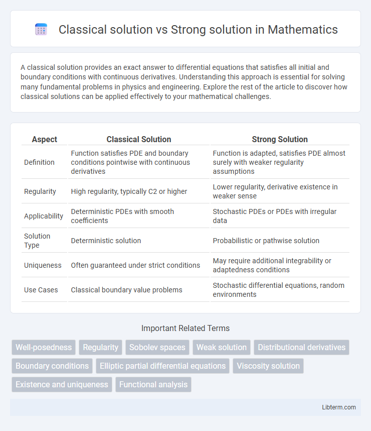
| Aspect | Classical Solution | Strong Solution |
|---|---|---|
| Definition | Function satisfies PDE and boundary conditions pointwise with continuous derivatives | Function is adapted, satisfies PDE almost surely with weaker regularity assumptions |
| Regularity | High regularity, typically C2 or higher | Lower regularity, derivative existence in weaker sense |
| Applicability | Deterministic PDEs with smooth coefficients | Stochastic PDEs or PDEs with irregular data |
| Solution Type | Deterministic solution | Probabilistic or pathwise solution |
| Uniqueness | Often guaranteed under strict conditions | May require additional integrability or adaptedness conditions |
| Use Cases | Classical boundary value problems | Stochastic differential equations, random environments |
Introduction to Classical and Strong Solutions
Classical solutions to partial differential equations require the function to be continuously differentiable enough times to satisfy the equation pointwise, ensuring strict adherence to the differential operator. Strong solutions relax these smoothness requirements, demanding less regularity by interpreting the differential equation in an integral or weak sense while still fulfilling the equation almost everywhere. Both solution concepts form the foundation for analyzing existence, uniqueness, and stability within PDE theory, with classical solutions emphasizing differentiability and strong solutions emphasizing integrability and weaker derivative interpretations.
Definition of Classical Solution
A classical solution to a partial differential equation (PDE) is a function that is sufficiently smooth, typically continuously differentiable as required by the equation, and satisfies the PDE pointwise in its domain. This contrasts with a strong solution, which may relax some regularity conditions and satisfy the PDE almost everywhere or in an integral sense. Classical solutions provide explicit, direct verification of the PDE and boundary conditions, ensuring strong analytical properties and uniqueness under standard assumptions.
Definition of Strong Solution
A strong solution to a stochastic differential equation (SDE) is defined as a solution process adapted to the filtration generated by a given Brownian motion, ensuring the solution is constructed on the same probability space as the driving noise. Unlike a classical (or weak) solution, where the probability space and Brownian motion can be chosen along with the process, a strong solution requires the pathwise uniqueness and measurability with respect to the original filtration. This concept is crucial for modeling systems where the randomness is predetermined and cannot be altered.
Mathematical Prerequisites
Classical solutions to partial differential equations require high regularity conditions, typically demanding functions to be continuously differentiable multiple times, ensuring the existence of all derivatives involved in the equation. Strong solutions relax these differentiability constraints by interpreting the PDE in an integral or weak form, relying on Sobolev spaces and weak derivatives to accommodate less regularity. The mathematical prerequisites for classical solutions emphasize smoothness and pointwise differentiability, whereas strong solutions depend on functional analysis tools like Sobolev spaces, weak derivatives, and variational formulations.
Existence and Uniqueness Criteria
Classical solutions to differential equations require the function to be continuously differentiable, ensuring existence and uniqueness under conditions like the Picard-Lindelof theorem, which demands Lipschitz continuity of the function. Strong solutions, often used in stochastic differential equations, exist when the solution is adapted to the filtration generated by the driving Brownian motion and satisfy integrability conditions guaranteeing uniqueness. Existence and uniqueness criteria for classical solutions primarily rely on smoothness and Lipschitz conditions, whereas strong solutions depend on probabilistic frameworks and measurability constraints.
Key Differences Between Classical and Strong Solutions
Classical solutions to partial differential equations require the function to be continuously differentiable enough to satisfy the equation pointwise, ensuring smoothness and explicit differentiability. Strong solutions relax these smoothness requirements by satisfying the equation almost everywhere in an integral or weak sense, allowing for less regularity while still maintaining essential solution properties. The key difference lies in the regularity and differentiability conditions imposed: classical solutions demand higher smoothness, whereas strong solutions accept functions with weaker differentiability but stronger integrability conditions.
Examples in Partial Differential Equations
Classical solutions to partial differential equations (PDEs) require the function to be continuously differentiable enough to satisfy the equation pointwise, such as the heat equation \( u_t = \alpha u_{xx} \) with smooth initial data. Strong solutions relax continuity requirements by interpreting derivatives in a weaker or distributional sense, exemplified by solutions to the Navier-Stokes equations where velocity fields have square-integrable derivatives. Examples like the Poisson equation \( -\Delta u = f \) illustrate classical solutions when \(f\) is smooth, while strong solutions emerge in Sobolev spaces when \(f\) belongs to \(L^2\)-spaces, allowing broader function classes.
Regularity Requirements and Function Spaces
Classical solutions to partial differential equations require high regularity, typically belonging to function spaces like \( C^2(\Omega) \) or Sobolev spaces \( W^{2,p}(\Omega) \), ensuring twice differentiability and pointwise satisfaction of the equation. Strong solutions relax the regularity demands, usually existing in Sobolev spaces \( W^{1,2}(\Omega) \) or \( H^1(\Omega) \), where derivatives are interpreted in a weak or distributional sense, allowing for solutions with less smoothness. The choice between classical and strong solutions depends on the PDE's complexity and boundary conditions, influencing the required function space and derivative interpretation.
Advantages and Limitations of Each Approach
Classical solutions provide explicit formulas for differential equations, offering precise and easily interpretable results ideal for smooth initial conditions; however, they often fail when equations involve irregularities or non-smooth data. Strong solutions extend applicability to less regular or stochastic settings by ensuring integrability and almost sure uniqueness yet may lack closed-form expressions and require more advanced mathematical frameworks. The classical approach excels in simplicity and intuition, whereas strong solutions enhance flexibility and robustness in complex, real-world modeling scenarios.
Applications and Practical Implications
Classical solutions, defined by smoothness and differentiability, are essential in deterministic models such as fluid dynamics and classical mechanics where precise boundary conditions are available. Strong solutions, which meet stochastic differential equations almost surely, are crucial for modeling systems influenced by randomness, like financial markets and weather forecasting. Understanding the distinction aids in selecting appropriate mathematical frameworks for accurate simulations and predictions in engineering, economics, and environmental sciences.
Classical solution Infographic