Stationarity refers to the property of a time series whose statistical characteristics, such as mean and variance, remain constant over time, making it crucial for reliable forecasting and modeling. Understanding stationarity helps in applying appropriate transformations to stabilize data and improve predictive accuracy. Explore the rest of the article to discover practical methods for testing and achieving stationarity in your time series analysis.
Table of Comparison
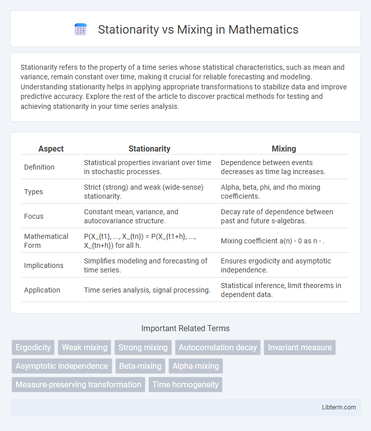
| Aspect | Stationarity | Mixing |
|---|---|---|
| Definition | Statistical properties invariant over time in stochastic processes. | Dependence between events decreases as time lag increases. |
| Types | Strict (strong) and weak (wide-sense) stationarity. | Alpha, beta, phi, and rho mixing coefficients. |
| Focus | Constant mean, variance, and autocovariance structure. | Decay rate of dependence between past and future s-algebras. |
| Mathematical Form | P(X_{t1}, ..., X_{tn}) = P(X_{t1+h}, ..., X_{tn+h}) for all h. | Mixing coefficient a(n) - 0 as n - . |
| Implications | Simplifies modeling and forecasting of time series. | Ensures ergodicity and asymptotic independence. |
| Application | Time series analysis, signal processing. | Statistical inference, limit theorems in dependent data. |
Introduction to Stationarity and Mixing
Stationarity in time series implies that statistical properties such as mean, variance, and autocorrelation remain constant over time, ensuring consistency in data behavior. Mixing conditions describe the dependence structure, quantifying how future values become increasingly independent of past values as time intervals grow. Understanding stationarity and mixing is essential for reliable modeling and inference in stochastic processes, as they influence convergence properties and the applicability of limit theorems.
Defining Stationarity in Time Series
Stationarity in time series refers to the property where statistical characteristics such as mean, variance, and autocorrelation remain constant over time, ensuring consistent behavior across different time intervals. Strict stationarity requires the joint distribution of any subset of observations to be invariant under time shifts, while weak stationarity only demands constancy in first and second moments. Understanding stationarity is crucial for modeling, forecasting, and inference since many time series analysis methods assume or require stationary data to produce valid results.
What is Mixing in Stochastic Processes?
Mixing in stochastic processes refers to a strong form of dependence decay where the future and past events become increasingly independent as the time gap between them grows. This property ensures that the joint distribution of events separated by a large lag approximates the product of their marginal distributions, enabling limit theorems and ergodic properties. Unlike stationarity, which implies consistent statistical structure over time, mixing quantifies how quickly correlations vanish, crucial for statistical inference in time series analysis.
Types of Stationarity: Strict vs. Weak
Strict stationarity requires that the joint distribution of any collection of time series values remains invariant under time shifts, ensuring a consistent probabilistic structure throughout the series. Weak stationarity, or covariance stationarity, imposes less stringent conditions, demanding only constant mean, constant variance, and autocovariance depending solely on lag rather than actual time points. Understanding these types is crucial for model selection and inference in time series analysis, where strict stationarity guarantees stronger stability while weak stationarity suffices for many practical applications involving linear models.
Different Mixing Conditions Explained
Mixing conditions describe the dependence structure of a stochastic process beyond stationarity, quantifying how quickly future and past events become independent as the time gap increases. Key mixing types include a-mixing (strong mixing), which measures the maximum dependency between s-algebras separated by time, b-mixing (absolute regularity), focusing on total variation distance, and ph-mixing, representing a stronger, more restrictive form of dependence decay. These conditions provide hierarchical control over temporal dependence, essential for establishing limit theorems in time series analysis and ergodic theory.
Stationarity and Mixing: Key Differences
Stationarity refers to a stochastic process whose statistical properties, such as mean and variance, remain constant over time, ensuring consistent behavior across different time intervals. Mixing, on the other hand, describes the property of a process where dependencies between past and future events diminish as the time gap increases, promoting statistical independence over long periods. The key difference lies in stationarity emphasizing time-invariant distributions, while mixing concentrates on the decay of correlations and dependencies over time.
Why Stationarity Matters in Statistical Analysis
Stationarity matters in statistical analysis because it ensures that the statistical properties of a process, such as mean and variance, remain constant over time, allowing for more reliable modeling and prediction. Non-stationary data can lead to spurious results and inaccurate inferences in time series analysis. Mixing conditions, which describe the dependence structure of data, complement stationarity by providing a framework for understanding the decay of correlations, crucial for hypothesis testing and consistency of estimators.
The Role of Mixing in Time Series Modeling
Mixing conditions in time series modeling provide a rigorous framework for quantifying dependence decay between distant observations, ensuring the validity of statistical inference methods under non-independent data. Stationarity guarantees constant probabilistic properties over time, but mixing strengthens this by controlling the rate at which dependence diminishes, allowing statistical estimators to achieve consistency and asymptotic normality. Models satisfying strong mixing conditions, such as a-mixing or b-mixing, facilitate effective estimation and hypothesis testing in autoregressive and moving average processes by ensuring ergodic behavior.
Applications: When to Use Stationarity or Mixing
Stationarity is essential for time series analysis where consistent statistical properties over time are required, such as in forecasting and econometrics models like ARIMA. Mixing conditions are preferred in situations demanding weak dependence assumptions, useful in proving limit theorems and ensuring reliable inference in high-frequency financial data or spatial statistics. Applying stationarity suits processes with stable distribution, while mixing is advantageous when dealing with more complex or evolving dependencies in data.
Conclusion: Choosing the Right Approach
Choosing between stationarity and mixing depends on the data's dependence structure and analysis goals. Stationarity assumes a stable distribution over time, ideal for modeling long-term trends, while mixing conditions accommodate more complex, dependent processes with weaker assumptions. Evaluating autocorrelation decay rates and model complexity ensures the selection of the approach that best captures temporal dependencies without compromising inference reliability.
Stationarity Infographic