Quadratic equations form the backbone of many mathematical models, describing parabolic shapes and solving complex problems in physics and engineering. Understanding the properties and solutions of quadratic functions empowers your ability to analyze real-world phenomena with precision. Explore the rest of the article to master quadratic concepts and their practical applications.
Table of Comparison
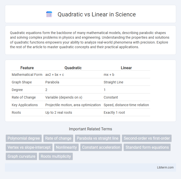
| Feature | Quadratic | Linear |
|---|---|---|
| Mathematical Form | ax2 + bx + c | mx + b |
| Graph Shape | Parabola | Straight Line |
| Degree | 2 | 1 |
| Rate of Change | Variable (depends on x) | Constant |
| Key Applications | Projectile motion, area optimization | Speed, distance-time relation |
| Roots | Up to 2 real roots | Exactly 1 root |
Introduction to Quadratic and Linear Functions
Quadratic functions are polynomial functions of degree two, typically expressed as f(x) = ax2 + bx + c, where a, b, and c are constants, and a 0. Linear functions, in contrast, are first-degree polynomials of the form f(x) = mx + b, representing straight lines with slope m and y-intercept b. Understanding the differences in their algebraic forms and corresponding graph shapes is essential for analyzing rates of change, curvature, and applications in physics, economics, and engineering.
Defining Linear Functions
Linear functions are mathematical expressions of the form f(x) = mx + b, where m represents the slope and b denotes the y-intercept, characterizing a constant rate of change. Unlike quadratic functions, which include an x2 term causing a curved graph, linear functions produce straight lines on the Cartesian plane. These functions model real-world phenomena with consistent, uniform growth or decline, making them essential in fields such as economics, physics, and engineering.
Understanding Quadratic Functions
Quadratic functions are mathematical expressions of the form f(x) = ax^2 + bx + c, where the highest degree of x is 2, distinguishing them from linear functions expressed as f(x) = mx + b. Understanding quadratic functions involves analyzing their parabolic graphs, vertex, axis of symmetry, and roots, which represent solutions to the equation ax^2 + bx + c = 0. Unlike linear functions with constant rates of change, quadratic functions exhibit variable rates of change due to their squared term, leading to more complex behavior in real-world applications like projectile motion and optimization problems.
Key Differences Between Quadratic and Linear Equations
Linear equations have the form y = mx + b, representing straight lines with a constant rate of change characterized by the slope m, while quadratic equations follow y = ax2 + bx + c, forming parabolic curves due to the squared variable x2. The key difference lies in their graph shapes: linear equations yield straight lines, whereas quadratic equations produce U-shaped parabolas that can open upward or downward depending on the sign of a. Linear equations have one root or solution, but quadratic equations can have two distinct, one repeated, or no real solutions based on the discriminant b2 - 4ac.
Graphical Representation: Linear vs Quadratic
Linear graphs depict straight lines characterized by a constant rate of change represented by the equation y = mx + b, where m is the slope and b is the y-intercept. Quadratic graphs form parabolas described by the equation y = ax^2 + bx + c, featuring a curved shape that opens upwards or downwards depending on the sign of the coefficient a. The vertex of a quadratic graph marks its maximum or minimum point, contrasting with the infinite extent and uniform slope of linear graphs.
Slope and Curvature: Linearity vs Parabolic Paths
Linear functions have a constant slope represented by a straight line, indicating uniform rate of change, while quadratic functions exhibit a variable slope that changes at each point along a parabolic curve. The curvature of a quadratic function is non-zero, causing the graph to bend either upwards or downwards, contrasting sharply with the zero curvature of linear functions. Understanding the distinction between the unchanging slope of linear models and the dynamically changing slope of quadratic models is essential for analyzing linearity versus parabolic trajectories in data or motion.
Real-Life Applications of Linear Functions
Linear functions model real-life situations where variables change at a constant rate, such as calculating speed, budgeting expenses, or predicting sales revenue. These functions simplify decision-making processes by providing straightforward relationships between independent and dependent variables. In contrast, quadratic functions suit scenarios involving acceleration or area, but linear models remain essential for daily financial planning and resource allocation.
Practical Uses of Quadratic Functions
Quadratic functions are essential in modeling real-world phenomena involving projectile motion, such as calculating the trajectory of a ball or optimizing the angle for maximum distance in sports. They are also employed in economics to find maximum profit or minimum cost by analyzing revenue and cost functions with parabolic graphs. Linear functions, in contrast, are more suited for problems requiring constant rates of change, like budgeting or speed, where relationships are proportional and graphs are straight lines.
Advantages and Limitations of Each Function
Quadratic functions offer the advantage of modeling nonlinear relationships with a parabolic curve, making them ideal for representing acceleration, projectile motion, and optimization problems. However, their complexity can lead to difficulty in solving and interpreting results compared to linear functions, which provide simplicity, ease of calculation, and straightforward interpretation due to their constant rate of change. Linear functions, while limited in capturing curvature and variable rates of change, excel in efficiency and applicability to scenarios with proportional relationships and consistent trends.
Choosing Between Quadratic and Linear for Problem-Solving
Choosing between quadratic and linear models depends on the nature of the problem and data behavior. Linear models are ideal for relationships with constant rates of change, offering simplicity and faster computation, especially in large datasets or real-time scenarios. Quadratic models capture curvature and variable rates of change, making them suitable for problems involving acceleration or maximum/minimum optimization, though they require more computational resources and complex interpretation.
Quadratic Infographic