The binomial distribution models the number of successes in a fixed number of independent Bernoulli trials with the same probability of success. It is widely used in statistics for calculating probabilities when outcomes are binary, such as success/failure or yes/no scenarios. Explore the rest of the article to understand how this distribution can be applied to your data analysis tasks effectively.
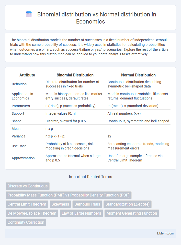
Table of Comparison
| Attribute | Binomial Distribution | Normal Distribution |
|---|---|---|
| Definition | Discrete distribution for number of successes in fixed trials | Continuous distribution describing symmetric bell-shaped data |
| Application in Economics | Models binary outcomes like market entry success, default rates | Models continuous variables like asset returns, demand fluctuations |
| Parameters | n (trials), p (success probability) | m (mean), s (standard deviation) |
| Support | Integer values [0, n] | All real numbers (-, +) |
| Shape | Discrete, skewed for p 0.5 | Continuous, symmetric and bell-shaped |
| Mean | n x p | m |
| Variance | n x p x (1 - p) | s2 |
| Use Case | Probability of k successes, risk modeling in credit decisions | Forecasting economic trends, modeling measurement errors |
| Approximation | Approximates Normal when n large and p 0.5 | Used for large sample inference via Central Limit Theorem |
Introduction to Probability Distributions
Binomial distribution models the number of successes in a fixed number of independent Bernoulli trials with a constant probability of success, often used for discrete random variables. Normal distribution describes continuous data with a symmetric bell-shaped curve characterized by its mean and standard deviation, representing natural variations around an average. Understanding these fundamental probability distributions enables accurate modeling and analysis of diverse random phenomena in statistics and data science.
Understanding Binomial Distribution
The binomial distribution models the probability of obtaining a fixed number of successes in a specific number of independent Bernoulli trials with the same probability of success, represented by parameters n (number of trials) and p (probability of success). It is discrete and often used in scenarios like quality control, clinical trials, and survey analysis, where outcomes are binary (success/failure). Understanding the binomial distribution helps in determining cumulative probabilities, expected value (np), and variance (np(1-p)), which are foundational for approximating the normal distribution when n is large and p is not too close to 0 or 1.
Key Properties of Binomial Distribution
The Binomial distribution models the number of successes in a fixed number of independent Bernoulli trials, each with the same probability of success p. Its key properties include discrete outcomes, a mean of np, and a variance of np(1-p), where n is the number of trials. The distribution is symmetric when p = 0.5 and skewed otherwise, approaching the Normal distribution as n increases, according to the Central Limit Theorem.
Introduction to Normal Distribution
The Normal distribution, also called the Gaussian distribution, is a continuous probability distribution characterized by its symmetric bell-shaped curve centered around the mean. It serves as an approximation to the Binomial distribution when the number of trials is large and the probability of success is neither too close to 0 nor 1, allowing the use of parameters mean (np) and variance (np(1-p)). The Normal distribution is fundamental in statistics due to the Central Limit Theorem, which states that sums of independent random variables tend toward a Normal distribution regardless of the original distribution.
Key Properties of Normal Distribution
The normal distribution exhibits a symmetric, bell-shaped curve characterized by its mean and standard deviation, with data evenly distributed around the mean. It is continuous, defined for all real numbers, and follows the empirical rule: approximately 68% of data falls within one standard deviation, 95% within two, and 99.7% within three standard deviations from the mean. Unlike the binomial distribution, which is discrete and based on a fixed number of trials, the normal distribution is often used as an approximation for large-sample binomial distributions due to the Central Limit Theorem.
Binomial vs Normal Distribution: Core Differences
The binomial distribution models the number of successes in a fixed number of independent Bernoulli trials with a constant probability, while the normal distribution describes continuous data with a symmetric bell curve characterized by its mean and standard deviation. Key differences include the binomial's discrete nature versus the normal's continuous range, and the normal distribution often serves as an approximation to the binomial when the number of trials is large and success probability is not too close to 0 or 1, applying the Central Limit Theorem. Variance in binomial distribution depends on both the number of trials and probability of success, whereas normal distribution variance is independent of trial structure.
Applicability: When to Use Binomial or Normal
The binomial distribution is ideal for modeling discrete events with fixed trials and two possible outcomes, such as success or failure, especially when the number of trials n is small and the probability of success p is known. The normal distribution is preferred for continuous data or large sample sizes where the binomial distribution's shape approximates normality, typically when np and n(1-p) are both greater than 5. Use the binomial distribution for exact probabilities in small samples and transition to the normal distribution as an efficient approximation for large sample binomial problems.
Relationship Between Binomial and Normal (Normal Approximation)
The binomial distribution, defined by parameters \(n\) (number of trials) and \(p\) (probability of success), approaches the normal distribution as \(n\) increases and \(p\) remains fixed, according to the Central Limit Theorem. When \(n\) is large and both \(np\) and \(n(1-p)\) exceed 5 or 10, the binomial distribution can be approximated by a normal distribution with mean \(\mu = np\) and variance \(\sigma^2 = np(1-p)\). This normal approximation simplifies calculation of binomial probabilities, especially for large sample sizes where exact binomial computations become cumbersome.
Real-World Examples and Applications
Binomial distribution models discrete events with fixed trials and outcomes, such as the number of defective products in a batch or success rates in clinical trials, providing precise probabilities for specific counts. Normal distribution applies to continuous data like heights, test scores, or measurement errors, enabling predictions about ranges and averages in large populations. Real-world use involves binomial in quality control and epidemiology, while normal distribution supports statistical inference and natural phenomena analysis.
Summary: Choosing the Right Distribution
Binomial distribution is ideal for modeling discrete events with fixed trials and constant success probability, such as pass/fail outcomes or yes/no surveys, while normal distribution suits continuous data with symmetric, bell-shaped patterns like heights or test scores. For large sample sizes, the binomial distribution approximates the normal distribution due to the Central Limit Theorem, simplifying calculations. Selecting the correct distribution depends on data type, sample size, and the requirement for discrete versus continuous analysis.
Binomial distribution Infographic