The Multinomial Logit model estimates the probability of different categorical outcomes based on multiple predictor variables, making it essential for analyzing choices with more than two discrete alternatives. This model assumes independence of irrelevant alternatives, meaning the odds between any two outcomes are unaffected by other available options. Explore the rest of the article to understand how this model can improve your decision-making analysis and practical applications.
Table of Comparison
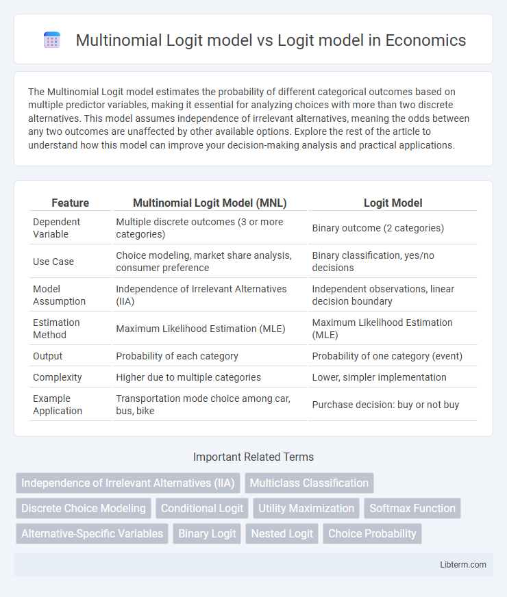
| Feature | Multinomial Logit Model (MNL) | Logit Model |
|---|---|---|
| Dependent Variable | Multiple discrete outcomes (3 or more categories) | Binary outcome (2 categories) |
| Use Case | Choice modeling, market share analysis, consumer preference | Binary classification, yes/no decisions |
| Model Assumption | Independence of Irrelevant Alternatives (IIA) | Independent observations, linear decision boundary |
| Estimation Method | Maximum Likelihood Estimation (MLE) | Maximum Likelihood Estimation (MLE) |
| Output | Probability of each category | Probability of one category (event) |
| Complexity | Higher due to multiple categories | Lower, simpler implementation |
| Example Application | Transportation mode choice among car, bus, bike | Purchase decision: buy or not buy |
Introduction to Logit and Multinomial Logit Models
Logit models estimate the probability of a binary outcome by modeling the log-odds as a linear function of predictor variables, commonly used in binary classification problems. Multinomial Logit models extend this approach to handle dependent variables with more than two categories by estimating probabilities for each outcome through multiple logit functions relative to a base category. Both models rely on the logistic distribution for error terms and are widely applied in fields like economics, marketing, and social sciences for discrete choice analysis.
Overview of the Logit Model
The Logit model estimates the probability of a binary outcome based on one or more predictor variables using the logistic function, making it ideal for dichotomous dependent variables. It transforms linear regression outputs through the logit link function to model odds, ensuring probabilities remain between 0 and 1. The Multinomial Logit model extends this framework to handle categorical dependent variables with more than two unordered outcomes, allowing comparison across multiple categories simultaneously.
Overview of the Multinomial Logit Model
The Multinomial Logit Model (MNL) extends the basic Logit model by accommodating dependent variables with more than two discrete outcomes, allowing for the analysis of choice among multiple alternatives. Unlike the binary Logit model, MNL estimates the probability of each category relative to a baseline category using a set of explanatory variables. This model is widely used in fields such as marketing, transportation, and economics for predicting outcomes like product choice, travel mode selection, or voting behavior.
Key Differences Between Logit and Multinomial Logit Models
The key differences between Logit and Multinomial Logit models lie in their application and outcome variable structure; the Logit model is used for binary outcome variables, modeling the probability of one of two categories, while the Multinomial Logit model handles dependent variables with three or more unordered categories. The Multinomial Logit model estimates separate logits for each outcome category relative to a baseline category, capturing the influence of predictor variables on multiple choice alternatives simultaneously. Logit models assume a simple dichotomy and utilize a logistic function for probability estimation, whereas Multinomial Logit models extend this framework to multiclass classification, enabling more complex discrete choice analysis.
Assumptions Underlying Each Model
The Multinomial Logit model assumes the independence of irrelevant alternatives (IIA), meaning the odds between any two choices are unaffected by the presence of other options, whereas the binary Logit model does not require this assumption as it involves only two alternatives. Both models assume a linear relationship between the predictors and the log-odds of the dependent variable, but the Multinomial Logit model extends this to multiple categories. Error terms in both models are assumed to be independently and identically distributed following the extreme value distribution, with the Multinomial Logit model requiring this across multiple outcome alternatives.
Mathematical Formulations: Logit vs Multinomial Logit
The Logit model is mathematically formulated using the logistic function to model binary outcomes with the probability \( P(Y=1) = \frac{e^{\beta'X}}{1 + e^{\beta'X}} \), while the Multinomial Logit (MNL) model generalizes this to multiple categories, representing probabilities as \( P(Y=j) = \frac{e^{\beta_j'X}}{\sum_{k=1}^J e^{\beta_k'X}} \) for \( j = 1, ..., J \). The MNL model requires estimating distinct coefficient vectors \( \beta_j \) for each category relative to a reference base outcome, accommodating situations with more than two discrete choices. In contrast, the Logit model estimates a single coefficient vector \( \beta \), making it suitable exclusively for binary classification tasks.
Use Cases and Applications
The Multinomial Logit (MNL) model is primarily used for predicting outcomes with more than two discrete categories, such as consumer product choice, transportation mode selection, and brand preference analysis, making it ideal for market research and behavioral modeling. The Logit model, or binary logit, is best suited for situations involving two possible outcomes, like credit approval decisions, medical diagnosis (disease vs. no disease), and binary classification problems in marketing campaigns. While both models estimate the probability of categorical outcomes, the MNL extends the binary Logit's utility to multi-class classification problems in economics, social sciences, and machine learning.
Model Estimation and Interpretation
The Multinomial Logit model estimates probabilities for outcomes with more than two categories by modeling the log-odds of each category relative to a baseline, whereas the binary Logit model handles only two possible outcomes. Parameter estimation in both models is typically performed using maximum likelihood estimation, but Multinomial Logit requires a more complex likelihood function due to multiple alternative categories. Interpretation of coefficients in the Multinomial Logit model involves comparing relative risk ratios for each category against the reference, while in the binary Logit model, coefficients reflect the change in log-odds for the single binary outcome.
Limitations and Considerations
The Multinomial Logit (MNL) model faces the Independence of Irrelevant Alternatives (IIA) limitation, which assumes that the relative odds between any two choices are unaffected by the presence of other options, potentially leading to biased estimates in correlated choice scenarios. In contrast, the binary Logit model is constrained to two outcome categories, limiting its application in multi-class classification problems. Careful consideration of the data structure and the assumption validity is essential when choosing between MNL and Logit models for accurate modeling of categorical dependent variables.
Choosing the Right Model for Your Data
Selecting the appropriate model depends on the nature of your dependent variable: use a Logit model for binary outcomes and a Multinomial Logit model when the dependent variable contains three or more unordered categories. The Multinomial Logit model extends the binary Logit framework to handle multiple discrete outcomes by estimating relative probabilities for each category. Accurate model choice improves predictive accuracy and interpretation in applications such as marketing segmentation, transportation mode choice, and healthcare decision analysis.
Multinomial Logit model Infographic