Stationarity refers to a statistical property of a time series where its mean, variance, and autocorrelation structure remain constant over time, ensuring consistent behavior for modeling and forecasting. Understanding stationarity is crucial in time series analysis to apply appropriate methods like ARIMA, which assume a stationary process. Explore the rest of this article to learn how to test for stationarity and transform your data for more accurate predictions.
Table of Comparison
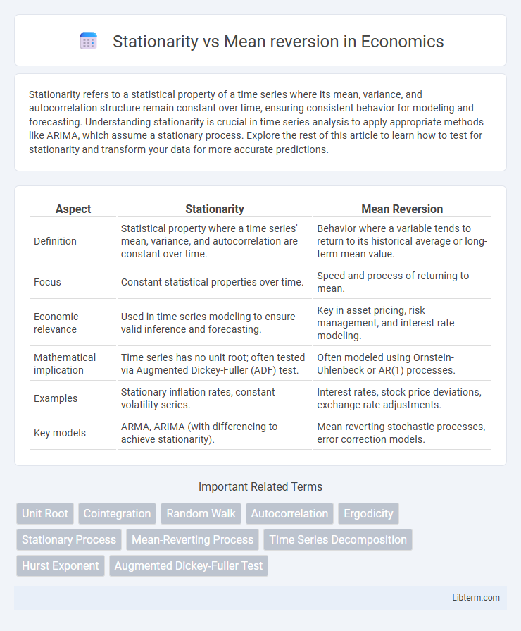
| Aspect | Stationarity | Mean Reversion |
|---|---|---|
| Definition | Statistical property where a time series' mean, variance, and autocorrelation are constant over time. | Behavior where a variable tends to return to its historical average or long-term mean value. |
| Focus | Constant statistical properties over time. | Speed and process of returning to mean. |
| Economic relevance | Used in time series modeling to ensure valid inference and forecasting. | Key in asset pricing, risk management, and interest rate modeling. |
| Mathematical implication | Time series has no unit root; often tested via Augmented Dickey-Fuller (ADF) test. | Often modeled using Ornstein-Uhlenbeck or AR(1) processes. |
| Examples | Stationary inflation rates, constant volatility series. | Interest rates, stock price deviations, exchange rate adjustments. |
| Key models | ARMA, ARIMA (with differencing to achieve stationarity). | Mean-reverting stochastic processes, error correction models. |
Understanding Stationarity in Time Series
Stationarity in time series refers to the statistical property where the mean, variance, and autocorrelation structure remain constant over time, enabling more reliable modeling and forecasting. Stationary processes allow for the application of various analytical techniques, such as autoregressive integrated moving average (ARIMA) models, as their properties do not change with time. Understanding stationarity is crucial for distinguishing between true mean reversion, where series fluctuate around a stable mean, and non-stationary trends that can mislead analysis and prediction.
Defining Mean Reversion: Key Concepts
Mean reversion refers to the financial theory that asset prices and historical returns eventually revert to their long-term average or mean level. This concept assumes that extreme deviations from the mean are temporary and that prices will return to a stable equilibrium over time. Stationarity is a related statistical property indicating that a time series' mean and variance remain constant, ensuring mean reversion can be effectively modeled and predicted.
Stationarity vs Mean Reversion: Core Differences
Stationarity refers to a time series property where statistical measures like mean and variance remain constant over time, ensuring predictable behavior. Mean reversion describes a process where values tend to return to a long-term average after deviations, indicating a pullback mechanism in data sequences. The core difference lies in stationarity being a broader characteristic of consistent distribution, while mean reversion specifically involves the tendency of a series to revert to its mean value.
Types of Stationarity in Data Analysis
Stationarity in data analysis refers to a statistical property where a time series' mean, variance, and autocorrelation structure do not change over time, which is crucial for reliable modeling and forecasting. Types of stationarity include strict stationarity, where the entire distribution is invariant over time, and weak stationarity, focusing on constant mean and autocovariance independent of time lag. Understanding these types helps distinguish stationary processes from mean-reverting ones, where data tends to revert to a long-term mean but may not meet strict stationarity conditions.
Mean Reversion Mechanisms Explained
Mean reversion mechanisms describe the tendency of asset prices or economic variables to return to their historical average or equilibrium value over time, driven by imbalance corrections in supply and demand or market inefficiencies. In contrast to non-stationary processes, mean-reverting time series exhibit statistically stable properties such as constant mean and variance, making them predictable in the long run. Understanding mean reversion is crucial for modeling financial markets, risk management, and developing trading strategies based on temporary deviations from average levels.
Statistical Tests for Stationarity
Statistical tests for stationarity, such as the Augmented Dickey-Fuller (ADF) test, Phillips-Perron (PP) test, and Kwiatkowski-Phillips-Schmidt-Shin (KPSS) test, are essential tools for distinguishing stationarity from mean reversion in time series analysis. The ADF and PP tests evaluate the null hypothesis of a unit root (non-stationarity), while the KPSS test assesses the null hypothesis of stationarity, providing a complementary check. Accurate identification of stationarity versus mean reversion through these tests guides model selection in econometrics, finance, and signal processing for reliable forecasting and inference.
Identifying Mean Reverting Processes
Mean reverting processes are characterized by a tendency to return to a long-term mean or equilibrium level, making them a subset of stationary time series with constant mean and variance over time. Identifying mean reversion involves statistical tests such as the Augmented Dickey-Fuller (ADF) test or the KPSS test, which assess stationarity by detecting whether shocks have temporary or permanent effects on the series. Models like the Ornstein-Uhlenbeck process and AR(1) with a coefficient less than one effectively capture mean reverting behavior, distinguishing these series from non-stationary random walks.
Real-World Examples: Stationarity and Mean Reversion
Stationarity describes time series data whose statistical properties, such as mean and variance, remain constant over time, exemplified by stable temperature records or consistent manufacturing processes. Mean reversion refers to the tendency of a variable, like stock prices or interest rates, to return to its historical average after deviations. Real-world cases include currency exchange rates, which fluctuate but often revert to long-term means, and commodity prices that exhibit cyclical recovery patterns, highlighting the practical importance of distinguishing between stationary and mean-reverting processes.
Implications for Forecasting and Modeling
Stationarity implies constant statistical properties over time, enabling reliable forecasting models based on historical data patterns. Mean reversion indicates that values tend to return to a long-term average, allowing models to predict future values by estimating equilibrium levels and adjustment speeds. Understanding these properties guides the selection of appropriate time series models, such as ARMA for stationary data or error correction models for mean-reverting series, improving forecast accuracy.
Practical Applications in Finance and Economics
Stationarity in time series ensures consistent statistical properties over time, essential for accurate financial modeling and risk management. Mean reversion, observed in asset prices and interest rates, underpins strategies like statistical arbitrage and bond yield prediction by exploiting the tendency of variables to return to long-term averages. Practical applications include portfolio optimization, algorithmic trading, and economic forecasting, where detecting stationarity and mean-reverting behavior improves decision-making and predictive accuracy.
Stationarity Infographic