The log-normal distribution is a probability distribution of a random variable whose logarithm is normally distributed, making it useful for modeling skewed data such as income, stock prices, or natural phenomena like particle sizes. Its properties include a positive-only range and a right-skewed shape, which capture the multiplicative effects of random variables better than the normal distribution. Explore the rest of this article to understand how the log-normal distribution applies to your data analysis and statistical modeling needs.
Table of Comparison
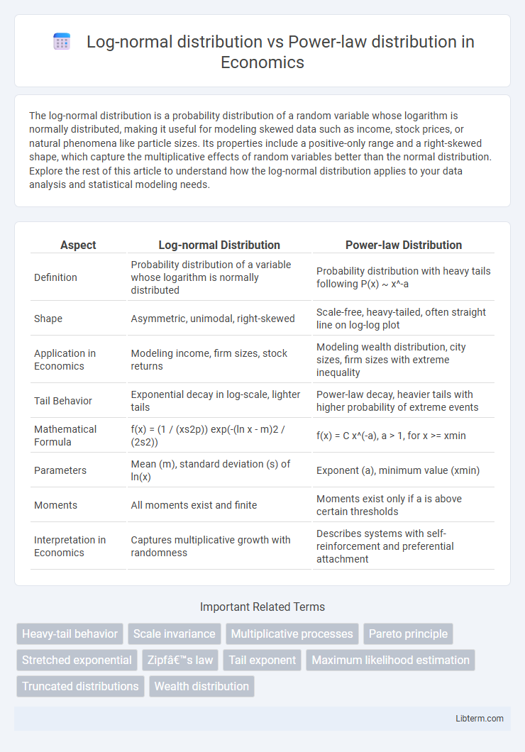
| Aspect | Log-normal Distribution | Power-law Distribution |
|---|---|---|
| Definition | Probability distribution of a variable whose logarithm is normally distributed | Probability distribution with heavy tails following P(x) ~ x^-a |
| Shape | Asymmetric, unimodal, right-skewed | Scale-free, heavy-tailed, often straight line on log-log plot |
| Application in Economics | Modeling income, firm sizes, stock returns | Modeling wealth distribution, city sizes, firm sizes with extreme inequality |
| Tail Behavior | Exponential decay in log-scale, lighter tails | Power-law decay, heavier tails with higher probability of extreme events |
| Mathematical Formula | f(x) = (1 / (xs2p)) exp(-(ln x - m)2 / (2s2)) | f(x) = C x^(-a), a > 1, for x >= xmin |
| Parameters | Mean (m), standard deviation (s) of ln(x) | Exponent (a), minimum value (xmin) |
| Moments | All moments exist and finite | Moments exist only if a is above certain thresholds |
| Interpretation in Economics | Captures multiplicative growth with randomness | Describes systems with self-reinforcement and preferential attachment |
Introduction to Statistical Distributions
Log-normal and power-law distributions represent two fundamental types of statistical distributions used to model complex phenomena. The log-normal distribution arises when the logarithm of the variable is normally distributed, often describing multiplicative processes and data with natural lower bounds. In contrast, power-law distributions characterize scale-invariant phenomena with heavy tails, capturing extreme events and underlying mechanisms like preferential attachment in networks.
Overview of Log-normal Distribution
The log-normal distribution describes a continuous probability distribution of a random variable whose logarithm is normally distributed, often modeling multiplicative processes and skewed data. It has a right-skewed shape characterized by parameters m (mean) and s (standard deviation) of the underlying normal distribution. Common applications include modeling financial asset prices, biological measurements, and income distributions, where values cannot be negative and exhibit long tails but with faster decay than power-law distributions.
Overview of Power-law Distribution
Power-law distribution describes a relationship where the frequency of an event scales as a power of its magnitude, often characterized by the probability density function \(P(x) \propto x^{-\alpha}\) for \(x \geq x_{\min}\), with \(\alpha\) as the scaling exponent. This distribution models phenomena with heavy tails and scale-invariance, commonly observed in natural and social systems such as earthquake magnitudes, wealth distribution, and network connectivity. Unlike the log-normal distribution, which arises from multiplicative processes and has a faster decaying tail, the power-law's tail decays polynomially, making extreme events significantly more probable.
Key Mathematical Properties
Log-normal distribution is characterized by a variable whose logarithm follows a normal distribution, resulting in a probability density function defined by parameters m and s representing the mean and standard deviation of the log-transformed variable. In contrast, the power-law distribution follows the form P(x) ~ x^(-a), where a > 1 is the scaling exponent dictating the heavy-tail behavior and scale invariance of phenomena such as wealth distribution or network connectivity. Unlike the log-normal's finite moments, the power-law distribution often has divergent higher moments depending on a, influencing the tail heaviness and risk modeling in complex systems.
Differences in Tail Behavior
Log-normal distribution tails decay exponentially, leading to thinner tails and fewer extreme values compared to power-law distribution. Power-law distribution features heavy tails with polynomial decay, resulting in a higher probability of extreme events and outliers. This fundamental difference impacts modeling in fields like finance and network theory, where tail risk and rare event occurrence are critical factors.
Real-world Applications and Examples
Log-normal distributions frequently model phenomena such as income distribution, stock market returns, and the sizes of living organisms, reflecting multiplicative growth processes. Power-law distributions describe systems with scale-invariance, commonly observed in earthquake magnitudes, city populations, and internet connectivity. Understanding these distinct patterns aids in risk assessment, resource allocation, and network resilience analysis across economics, geophysics, and information technology.
Methods for Distinguishing Log-normal and Power-law
Methods for distinguishing log-normal and power-law distributions primarily involve statistical goodness-of-fit tests such as the Kolmogorov-Smirnov test and likelihood ratio tests, which compare the fit of empirical data to both models. Maximum likelihood estimation (MLE) is applied to estimate parameters, followed by hypothesis testing to assess model suitability and tail behavior differences. Visual tools like log-log plots can provide initial clues, but rigorous model comparison metrics, including Akaike Information Criterion (AIC) and Bayesian Information Criterion (BIC), offer more reliable discrimination between log-normal and power-law distributions.
Visualization and Fitting Techniques
Visualizing Log-normal distribution often involves plotting data on a logarithmic scale, revealing a characteristic bell curve indicative of multiplicative processes, while Power-law distribution visualizations typically display linear behavior on log-log plots, highlighting scale-invariance in heavy-tailed data. Fitting Log-normal distributions utilizes maximum likelihood estimation (MLE) to estimate parameters such as the mean and standard deviation of the underlying normal distribution, ensuring accurate modeling of skewed data. Power-law fitting relies on methods like the Clauset-Shalizi-Newman approach with Kolmogorov-Smirnov statistics and likelihood ratio tests to robustly determine the scaling exponent and validate the presence of heavy tails versus alternative distributions.
Common Misconceptions and Pitfalls
Log-normal distribution is often mistaken for power-law distribution due to their similar heavy-tailed behavior, but log-normal tails decay faster, which affects the probability of extreme events. Misinterpreting data with limited scale ranges can lead to falsely identifying a power-law when the underlying distribution is actually log-normal. Statistical tests such as the Kolmogorov-Smirnov test or likelihood ratio tests are crucial to avoid these pitfalls and accurately distinguish between the two distributions.
Conclusion: Choosing the Right Distribution
Selecting between a log-normal distribution and a power-law distribution depends on the data's tail behavior and underlying generative processes. Log-normal distributions model data with multiplicative factors and exhibit thinner tails, suitable for scenarios with natural cutoffs, while power-law distributions capture heavy-tailed phenomena with scale-invariance, reflecting systems with infinite variance or self-organized criticality. Accurate model selection improves predictions, risk assessment, and understanding of complex systems by aligning statistical properties with empirical observations.
Log-normal distribution Infographic