The Linear Probability Model (LPM) is a straightforward approach to estimate binary outcome variables using linear regression techniques, providing easy-to-interpret coefficients that represent the change in probability associated with predictors. Despite its simplicity, the LPM can produce predicted probabilities outside the 0 to 1 range and may suffer from heteroskedasticity, making alternative methods like logistic regression preferable in many cases. Explore the rest of the article to understand when and how to effectively apply the Linear Probability Model in your analyses.
Table of Comparison
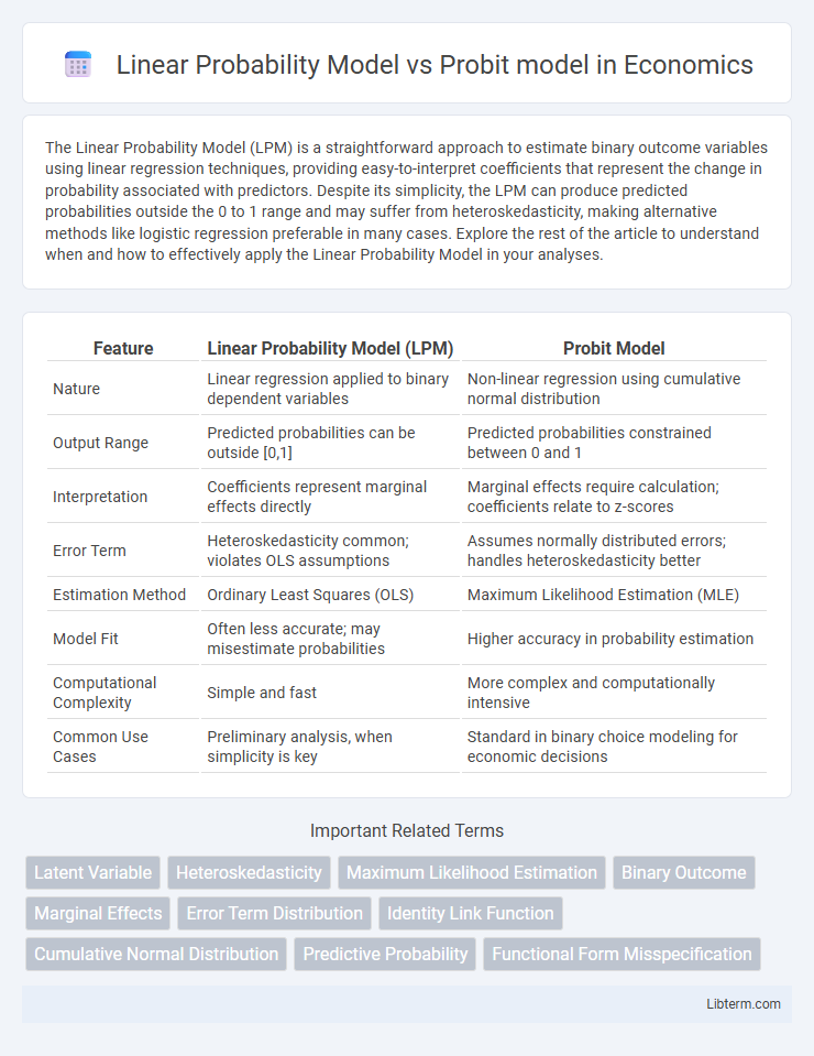
| Feature | Linear Probability Model (LPM) | Probit Model |
|---|---|---|
| Nature | Linear regression applied to binary dependent variables | Non-linear regression using cumulative normal distribution |
| Output Range | Predicted probabilities can be outside [0,1] | Predicted probabilities constrained between 0 and 1 |
| Interpretation | Coefficients represent marginal effects directly | Marginal effects require calculation; coefficients relate to z-scores |
| Error Term | Heteroskedasticity common; violates OLS assumptions | Assumes normally distributed errors; handles heteroskedasticity better |
| Estimation Method | Ordinary Least Squares (OLS) | Maximum Likelihood Estimation (MLE) |
| Model Fit | Often less accurate; may misestimate probabilities | Higher accuracy in probability estimation |
| Computational Complexity | Simple and fast | More complex and computationally intensive |
| Common Use Cases | Preliminary analysis, when simplicity is key | Standard in binary choice modeling for economic decisions |
Introduction to Linear Probability Model and Probit Model
The Linear Probability Model (LPM) estimates binary outcomes using a simple linear regression framework, interpreting predicted values directly as probabilities, although it may produce predictions outside the [0,1] range. The Probit model addresses this limitation by employing a cumulative normal distribution function to constrain predicted probabilities between 0 and 1, providing a more theoretically sound approach for modeling binary dependent variables. Both models serve as fundamental tools in binary choice analysis, with the Probit model offering better handling of nonlinear relationships inherent in probability data.
Fundamental Concepts of Binary Choice Models
Binary choice models analyze decisions with two possible outcomes, using different approaches to estimate probabilities. The Linear Probability Model (LPM) applies ordinary least squares to predict binary outcomes but can produce predictions outside the [0,1] range and assumes constant error variance, which may lead to inefficiency. The Probit model, grounded in the cumulative normal distribution, ensures predicted probabilities fall within the [0,1] interval and accounts for non-linear relationships by modeling latent variables underlying observed binary responses.
Mathematical Formulation of the Linear Probability Model
The Linear Probability Model (LPM) mathematically expresses the probability of a binary outcome as a linear function of independent variables using the equation P(Y=1|X) = Xb, where Y is the binary dependent variable, X represents explanatory variables, and b denotes the parameter vector. Unlike the Probit model, which applies a cumulative distribution function to ensure probabilities lie between 0 and 1, the LPM can yield predicted probabilities outside this range due to its linear specification. Despite its simplicity and ease of interpretation, LPM's mathematical formulation is limited by heteroscedasticity and non-normal error terms, challenging the reliability of standard inference methods.
Mathematical Formulation of the Probit Model
The Probit model mathematically expresses the probability of a binary outcome as \( P(Y=1|X) = \Phi(X\beta) \), where \( \Phi \) denotes the cumulative distribution function (CDF) of the standard normal distribution, modeling the latent variable's threshold crossing. This contrasts with the Linear Probability Model (LPM), which linearly estimates probabilities as \( P(Y=1|X) = X\beta \) without restricting the predicted values to the [0,1] interval. The Probit model ensures predicted probabilities remain within valid bounds through the nonlinear transformation of the normal CDF, providing a theoretically sound approach for binary dependent variables.
Assumptions Underlying Each Model
The Linear Probability Model (LPM) assumes a linear relationship between independent variables and the probability of a binary outcome, treating errors as homoscedastic and uncorrelated. The Probit model assumes that the latent variable follows a standard normal distribution, with errors normally distributed and the cumulative distribution function mapping to probabilities between 0 and 1. LPM's assumptions often lead to predicted probabilities outside the [0,1] range, while Probit ensures probabilities remain bounded and accounts for heteroscedasticity in error terms.
Advantages of the Linear Probability Model
The Linear Probability Model (LPM) offers simplicity and ease of interpretation since it uses ordinary least squares (OLS) regression, allowing direct estimation of marginal effects without complex transformations. It provides computational efficiency and straightforward implementation for binary dependent variables, making it useful for preliminary analysis or large datasets. The LPM's coefficients represent immediate probability changes, facilitating intuitive insights compared to Probit models, which require inverse normal cumulative distribution functions.
Advantages of the Probit Model
The Probit model offers significant advantages over the Linear Probability Model by providing predicted probabilities strictly within the 0 to 1 range, ensuring valid interpretations for binary outcome predictions. Its nonlinear approach captures the underlying latent variable structure more accurately, leading to better estimation of marginal effects and model fit for dichotomous dependent variables. Furthermore, the Probit model's assumption of normally distributed error terms aligns with many real-world phenomena, improving its applicability in fields like economics and biostatistics.
Limitations and Drawbacks: LPM vs Probit
The Linear Probability Model (LPM) suffers from heteroscedasticity and can predict probabilities outside the [0,1] interval, limiting its interpretability and reliability. In contrast, the Probit model addresses these issues by using a cumulative normal distribution, providing predicted probabilities strictly between 0 and 1 and accommodating the non-linear relationship between independent variables and the binary outcome. However, the Probit model is computationally more complex and requires assumptions about the error term distribution, making it less straightforward than the LPM for practical applications.
Practical Applications and Model Selection
Linear Probability Models (LPM) offer straightforward interpretation and simpler calculation of marginal effects, making them suitable for large datasets or initial exploratory analysis in binary outcome predictions. Probit models provide a more realistic estimation of probabilities within the (0,1) interval and are preferred when accuracy in capturing the nonlinear relationship between predictors and the probability of an event is critical. Model selection depends on the trade-off between computational simplicity and the need for precise probability estimates, with Probit favored in fields like finance and epidemiology where prediction accuracy influences decision-making.
Conclusion: Choosing Between LPM and Probit Model
Choosing between the Linear Probability Model (LPM) and Probit model depends on the nature of the dependent variable and the desired accuracy in estimating probabilities. The LPM offers simplicity and ease of interpretation but may suffer from heteroscedasticity and predicted probabilities outside the [0,1] range. The Probit model provides more precise probability estimates with a nonlinear functional form that respects the bounded probability scale, making it preferable for modeling binary outcomes when accuracy is critical.
Linear Probability Model Infographic