Jacobi polynomials form a class of orthogonal polynomials vital in numerical analysis and solving differential equations, characterized by two parameters that adjust their weight function. These polynomials generalize many other families, such as Legendre and Chebyshev polynomials, making them versatile tools in approximation theory and mathematical physics. Explore the full article to understand how Jacobi polynomials can enhance your computational methods.
Table of Comparison
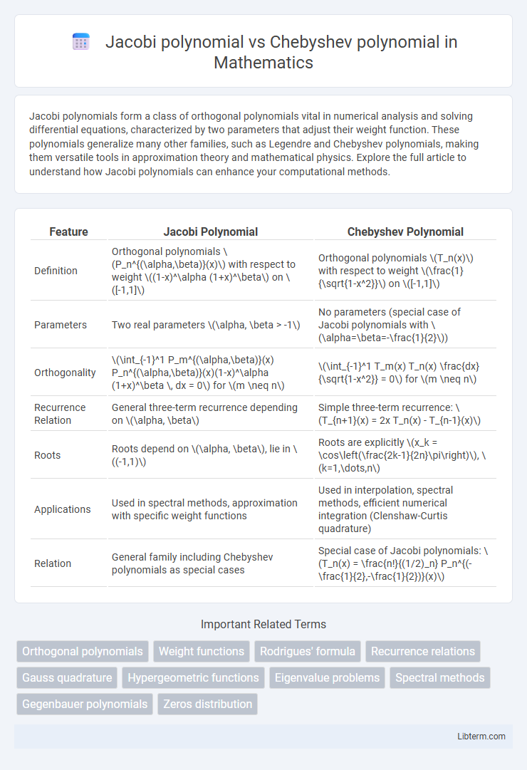
| Feature | Jacobi Polynomial | Chebyshev Polynomial |
|---|---|---|
| Definition | Orthogonal polynomials \(P_n^{(\alpha,\beta)}(x)\) with respect to weight \((1-x)^\alpha (1+x)^\beta\) on \([-1,1]\) | Orthogonal polynomials \(T_n(x)\) with respect to weight \(\frac{1}{\sqrt{1-x^2}}\) on \([-1,1]\) |
| Parameters | Two real parameters \(\alpha, \beta > -1\) | No parameters (special case of Jacobi polynomials with \(\alpha=\beta=-\frac{1}{2}\)) |
| Orthogonality | \(\int_{-1}^1 P_m^{(\alpha,\beta)}(x) P_n^{(\alpha,\beta)}(x)(1-x)^\alpha (1+x)^\beta \, dx = 0\) for \(m \neq n\) | \(\int_{-1}^1 T_m(x) T_n(x) \frac{dx}{\sqrt{1-x^2}} = 0\) for \(m \neq n\) |
| Recurrence Relation | General three-term recurrence depending on \(\alpha, \beta\) | Simple three-term recurrence: \(T_{n+1}(x) = 2x T_n(x) - T_{n-1}(x)\) |
| Roots | Roots depend on \(\alpha, \beta\), lie in \((-1,1)\) | Roots are explicitly \(x_k = \cos\left(\frac{2k-1}{2n}\pi\right)\), \(k=1,\dots,n\) |
| Applications | Used in spectral methods, approximation with specific weight functions | Used in interpolation, spectral methods, efficient numerical integration (Clenshaw-Curtis quadrature) |
| Relation | General family including Chebyshev polynomials as special cases | Special case of Jacobi polynomials: \(T_n(x) = \frac{n!}{(1/2)_n} P_n^{(-\frac{1}{2},-\frac{1}{2})}(x)\) |
Introduction to Orthogonal Polynomials
Jacobi polynomials form a class of classical orthogonal polynomials defined on the interval [-1, 1] with a weight function (1-x)^a(1+x)^b, characterized by two parameters a and b that control their shape and orthogonality. Chebyshev polynomials are a specific case of Jacobi polynomials with parameters a = b = -1/2, known for their minimization of polynomial approximation error and roots used in numerical methods like Gaussian quadrature. Both polynomial families serve as fundamental tools in approximation theory, spectral methods, and solving differential equations due to their orthogonality properties and explicit recurrence relations.
Overview of Jacobi Polynomials
Jacobi polynomials \(P_n^{(\alpha,\beta)}(x)\) form a family of classical orthogonal polynomials defined on the interval \([-1, 1]\) with respect to the weight function \((1-x)^\alpha (1+x)^\beta\), where \(\alpha, \beta > -1\). These polynomials generalize several important polynomial families, including Legendre polynomials (when \(\alpha=\beta=0\)) and Chebyshev polynomials (special cases of Jacobi polynomials with specific parameter values). Jacobi polynomials satisfy a second-order differential equation and possess rich properties in approximation theory, spectral methods, and numerical integration.
Overview of Chebyshev Polynomials
Chebyshev polynomials, a special case of Jacobi polynomials with parameters a = b = -1/2, play a fundamental role in approximation theory due to their minimax property and roots clustering at the endpoints of the interval [-1,1]. These polynomials, defined as T_n(x) = cos(n arccos x), are orthogonal with respect to the weight function (1 - x^2)^(-1/2), enabling efficient numerical methods for interpolation and spectral methods. Their explicit trigonometric form and stable recurrence relations make Chebyshev polynomials highly practical for minimizing Runge's phenomenon and achieving near-optimal polynomial approximations.
Mathematical Definitions and Notations
Jacobi polynomials \( P_n^{(\alpha,\beta)}(x) \) are a class of orthogonal polynomials defined on the interval \([-1,1]\) with weight function \( (1-x)^\alpha (1+x)^\beta \), where \( \alpha, \beta > -1 \), satisfying the differential equation \((1-x^2) y'' + [\beta-\alpha - (\alpha+\beta+2)x] y' + n(n+\alpha+\beta+1) y = 0\). Chebyshev polynomials of the first kind, \( T_n(x) \), are a specific case of Jacobi polynomials with parameters \( \alpha = \beta = -\frac{1}{2} \), explicitly defined by the recurrence \( T_0(x) = 1, T_1(x) = x, \) and \( T_{n+1}(x) = 2x T_n(x) - T_{n-1}(x) \). Both polynomial families are orthogonal, but Jacobi polynomials offer greater generality through parameters \(\alpha, \beta\), allowing for customized weight functions and applications in spectral methods.
Weight Functions and Orthogonality
Jacobi polynomials \( P_n^{(\alpha,\beta)}(x) \) are orthogonal on the interval \([-1, 1]\) with respect to the weight function \( (1-x)^\alpha (1+x)^\beta \), where \(\alpha, \beta > -1\), ensuring a flexible family of weight functions that include varying endpoint behaviors. Chebyshev polynomials of the first kind \( T_n(x) \) correspond to the Jacobi polynomials with \(\alpha = \beta = -\frac{1}{2}\), having the weight function \( \frac{1}{\sqrt{1-x^2}} \), and are orthogonal under this singular weight emphasizing endpoints. The orthogonality conditions for Jacobi polynomials produce a broad class of polynomial solutions critical for spectral methods, while Chebyshev polynomials provide efficient numerical stability and convergence properties due to their specific weight and simpler recursion relations.
Recurrence Relations Comparison
Jacobi polynomials \(P_n^{(\alpha,\beta)}(x)\) satisfy the three-term recurrence relation: \[ 2(n+1)(n+\alpha+\beta+1)(2n+\alpha+\beta) P_{n+1}^{(\alpha,\beta)}(x) = (2n+\alpha+\beta+1)\left[(2n+\alpha+\beta)(2n+\alpha+\beta+2)x + \alpha^2 - \beta^2\right] P_n^{(\alpha,\beta)}(x) - 2(n+\alpha)(n+\beta)(2n+\alpha+\beta+2) P_{n-1}^{(\alpha,\beta)}(x). \] Chebyshev polynomials of the first kind \(T_n(x)\) have a simpler recurrence: \[ T_{n+1}(x) = 2x T_n(x) - T_{n-1}(x), \] demonstrating that Jacobi polynomials generalize Chebyshev polynomials with additional parameters \(\alpha, \beta\) impacting the recurrence coefficients and orthogonality weight functions.
Applications in Numerical Analysis
Jacobi polynomials are widely used in numerical analysis for solving differential equations and spectral methods due to their flexibility in adjusting parameters to model various boundary conditions. Chebyshev polynomials, a special case of Jacobi polynomials, excel in polynomial approximation and interpolation tasks, minimizing Runge's phenomenon and improving convergence rates. Both polynomial families play critical roles in quadrature rules, with Gauss-Jacobi and Gauss-Chebyshev quadratures providing efficient numerical integration techniques.
Computational Efficiency and Stability
Jacobi polynomials exhibit greater computational flexibility due to their two-parameter family, allowing fine-tuning for specific weight functions, but this often leads to increased complexity in evaluation compared to Chebyshev polynomials. Chebyshev polynomials are known for their exceptional computational efficiency and numerical stability, particularly in iterative methods like polynomial approximation and spectral methods, due to simple recurrence relations and well-conditioned properties. Consequently, Chebyshev polynomials are generally preferred in applications demanding fast convergence and minimal numerical errors, while Jacobi polynomials are favored when custom weightings are essential despite higher computational costs.
Graphical Representation and Zeros
Jacobi polynomials exhibit varied shapes and zero distributions depending on their a and b parameters, with zeros concentrated more towards the interval endpoints for larger parameter values. Chebyshev polynomials of the first kind display a distinct oscillatory pattern with evenly spaced zeros in the interval [-1,1], corresponding to the cosine function roots. Graphically, Chebyshev polynomials present a smooth, near-minimax approximation curve, while Jacobi polynomials offer more flexibility in shape and zero placement due to their two-parameter weighting.
Choosing Between Jacobi and Chebyshev Polynomials
Choosing between Jacobi and Chebyshev polynomials depends on the specific weight functions and boundary conditions of the problem. Jacobi polynomials offer greater generality with parameters \(\alpha\) and \(\beta\), making them suitable for weighted inner products and custom orthogonality domains. Chebyshev polynomials, a special case of Jacobi polynomials with fixed parameters, provide computational simplicity and are ideal for approximation problems on the interval \([-1, 1]\) with uniform weighting.
Jacobi polynomial Infographic