Laguerre polynomials are solutions to Laguerre's differential equation and widely used in physics, particularly in quantum mechanics for solving the radial part of the Schrodinger equation. These orthogonal polynomials play a crucial role in numerical analysis and approximation theory due to their unique weighting functions. Explore the rest of this article to discover how Laguerre polynomials impact various scientific and engineering applications.
Table of Comparison
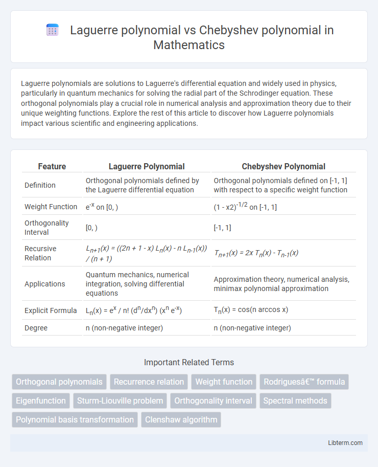
| Feature | Laguerre Polynomial | Chebyshev Polynomial |
|---|---|---|
| Definition | Orthogonal polynomials defined by the Laguerre differential equation | Orthogonal polynomials defined on [-1, 1] with respect to a specific weight function |
| Weight Function | e-x on [0, ) | (1 - x2)-1/2 on [-1, 1] |
| Orthogonality Interval | [0, ) | [-1, 1] |
| Recursive Relation | Ln+1(x) = ((2n + 1 - x) Ln(x) - n Ln-1(x)) / (n + 1) | Tn+1(x) = 2x Tn(x) - Tn-1(x) |
| Applications | Quantum mechanics, numerical integration, solving differential equations | Approximation theory, numerical analysis, minimax polynomial approximation |
| Explicit Formula | Ln(x) = ex / n! (dn/dxn) (xn e-x) | Tn(x) = cos(n arccos x) |
| Degree | n (non-negative integer) | n (non-negative integer) |
Introduction to Orthogonal Polynomials
Laguerre polynomials and Chebyshev polynomials are fundamental families of orthogonal polynomials used extensively in numerical analysis and approximation theory. Laguerre polynomials, defined on the interval [0, ), are orthogonal with respect to the weight function e^(-x), playing a key role in quantum mechanics and solving differential equations involving exponential decay. Chebyshev polynomials, orthogonal on the interval [-1, 1] with weight function (1-x^2)^(-1/2), are crucial for minimizing errors in polynomial interpolation and serve as a basis in spectral methods for solving differential equations.
Overview of Laguerre Polynomials
Laguerre polynomials are solutions to Laguerre's differential equation, widely used in quantum mechanics and numerical analysis for approximating functions on the interval [0, ). These polynomials form an orthogonal set with respect to the weight function e^(-x), distinguishing them from Chebyshev polynomials that are orthogonal on the interval [-1, 1] with weight function (1-x^2)^(-1/2). Their recurrence relations and generating functions facilitate efficient computation, making Laguerre polynomials essential tools in solving problems involving exponential decay and radial components in hydrogen-like atoms.
Overview of Chebyshev Polynomials
Chebyshev polynomials, defined by the recurrence relation T_n(x) = 2x T_{n-1}(x) - T_{n-2}(x) with T_0(x)=1 and T_1(x)=x, are widely used in approximation theory and numerical analysis for minimizing errors in polynomial interpolation. Unlike Laguerre polynomials, which are orthogonal on the interval [0, ) with weight function e^{-x}, Chebyshev polynomials are orthogonal on the interval [-1, 1] with the weight function (1 - x^2)^{-1/2}. Their extremal properties and minimax characteristics make Chebyshev polynomials essential in designing efficient algorithms for spectral methods and solving differential equations.
Mathematical Definitions and Formulations
Laguerre polynomials \(L_n^{(\alpha)}(x)\) are defined by the Rodrigues formula \(L_n^{(\alpha)}(x) = \frac{x^{-\alpha} e^x}{n!} \frac{d^n}{dx^n} (e^{-x} x^{n+\alpha})\), used primarily in solving differential equations with exponential weights. Chebyshev polynomials \(T_n(x)\), defined by the recurrence \(T_{n+1}(x) = 2x T_n(x) - T_{n-1}(x)\) with \(T_0(x)=1\) and \(T_1(x)=x\), are orthogonal on the interval \([-1,1]\) with weight \(\frac{1}{\sqrt{1-x^2}}\). Both sets belong to the family of classical orthogonal polynomials satisfying specific second-order linear differential equations important in approximation theory and numerical analysis.
Orthogonality Properties Compared
Laguerre polynomials are orthogonal with respect to the weight function \(e^{-x}\) on the interval \([0, \infty)\), making them suitable for problems involving exponential decay and quantum mechanics. Chebyshev polynomials, orthogonal on \([-1, 1]\) with the weight \((1-x^2)^{-1/2}\), are optimal for minimizing errors in polynomial approximation and numerical interpolation. The distinct weight functions and orthogonality intervals highlight their specific applications in spectral methods and approximation theory.
Recurrence Relations: Laguerre vs Chebyshev
Laguerre polynomials \(L_n^{(\alpha)}(x)\) satisfy the recurrence relation \( (n+1)L_{n+1}^{(\alpha)}(x) = (2n + \alpha + 1 - x)L_n^{(\alpha)}(x) - (n + \alpha)L_{n-1}^{(\alpha)}(x) \), emphasizing dependence on parameter \(\alpha\) and the variable \(x\). Chebyshev polynomials of the first kind \(T_n(x)\) follow the simpler recurrence \( T_{n+1}(x) = 2xT_n(x) - T_{n-1}(x) \), highlighting a direct linear relation without additional parameters. The distinct recurrence structures reflect their orthogonality on different intervals, with Laguerre polynomials orthogonal on \([0,\infty)\) weighted by \(e^{-x}x^\alpha\) and Chebyshev polynomials on \([-1,1]\) weighted uniformly.
Weight Functions and Interval Domains
Laguerre polynomials are orthogonal with respect to the weight function \( e^{-x} \) on the interval \([0, \infty)\), making them suitable for problems involving exponential decay and quantum mechanics. Chebyshev polynomials of the first kind, on the other hand, use the weight function \( \frac{1}{\sqrt{1-x^2}} \) and are orthogonal on the finite interval \([-1, 1]\), which is ideal for approximation theory in bounded domains. The distinct weight functions and interval domains define their orthogonality properties and determine their application in numerical analysis and spectral methods.
Applications in Numerical Methods
Laguerre polynomials are extensively used in numerical methods for solving differential equations with boundary conditions extending to infinity, making them ideal for quantum mechanics and signal processing applications. Chebyshev polynomials excel in polynomial approximation, interpolation, and spectral methods due to their minimization of Runge's phenomenon and optimal node distribution on the interval [-1,1]. Both polynomials enhance numerical stability and convergence rates in computational algorithms, with Laguerre polynomials suited for problems involving exponential weight functions and Chebyshev polynomials favored in spectral collocation and Fast Fourier Transform algorithms.
Computational Advantages and Limitations
Laguerre polynomials offer computational advantages in solving differential equations with exponential weight functions due to their orthogonality over the semi-infinite interval [0, ), making them suitable for problems in quantum mechanics and optics. Chebyshev polynomials provide efficient numerical stability and fast convergence in polynomial approximations and interpolation on the finite interval [-1, 1], leveraging their minimax property to reduce Runge's phenomenon. However, Laguerre polynomials may face slower convergence for non-exponential weight functions, while Chebyshev polynomials are less effective in handling problems defined on unbounded domains.
Choosing Between Laguerre and Chebyshev Polynomials
Choosing between Laguerre and Chebyshev polynomials depends on the problem domain and weight functions involved. Laguerre polynomials are optimal for functions defined on the positive real axis with an exponential decay weight, commonly used in quantum mechanics and signal processing for problems involving exponential decay or growth. Chebyshev polynomials excel in polynomial approximation on the interval [-1, 1] with a weight function of (1-x2)^(-1/2), making them ideal for minimizing the maximum error in numerical analysis and spectral methods.
Laguerre polynomial Infographic