A local minimum refers to a point in a function where the value is lower than all nearby points, representing a trough within a specific region of the graph. Understanding local minima is crucial in fields like optimization and machine learning to identify stable solutions and avoid suboptimal results. Explore the rest of the article to deepen Your understanding of local minima and their practical applications.
Table of Comparison
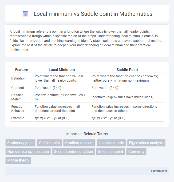
| Feature | Local Minimum | Saddle Point |
|---|---|---|
| Definition | Point where the function value is lower than all nearby points | Point where the function changes concavity; neither purely minimum nor maximum |
| Gradient | Zero vector (f = 0) | Zero vector (f = 0) |
| Hessian Matrix | Positive definite (all eigenvalues > 0) | Indefinite (eigenvalues have mixed signs) |
| Function Behavior | Function value increases in all directions around the point | Function value increases in some directions and decreases in others |
| Example | f(x, y) = x2 + y2 at (0, 0) | f(x, y) = x2 - y2 at (0, 0) |
Definition of Local Minimum
A local minimum is a point on a function where the value is lower than all nearby points, indicating a small neighborhood around it where the function does not decrease further. Unlike saddle points, which can be stationary points with higher values in one direction and lower values in another, a local minimum always exhibits non-negative curvature in its vicinity. Mathematically, a local minimum occurs where the gradient is zero and the Hessian matrix is positive semi-definite.
Definition of Saddle Point
A saddle point is a critical point on a surface where the slope is zero but does not represent a local minimum or maximum, resembling a "saddle" shape with curvature changing sign in different directions. Unlike local minima where the function value is lower than in surrounding points, a saddle point exhibits a mix of concave and convex curvatures, causing the point to be stable in one direction and unstable in another. This characteristic makes saddle points fundamental in optimization and differential geometry for understanding function behavior in multidimensional spaces.
Key Differences Between Local Minimum and Saddle Point
A local minimum is a point where the function value is lower than at any nearby points, indicating a stable equilibrium with positive definite Hessian matrix. A saddle point is a critical point where the function exhibits both convex and concave behavior in different directions, characterized by an indefinite Hessian matrix. Unlike local minima, saddle points do not represent a stable solution in optimization problems due to the presence of directions of descent and ascent.
Mathematical Representation
A local minimum of a function \( f(x) \) is a point \( x_0 \) where \( f(x_0) \leq f(x) \) for all \( x \) in a neighborhood around \( x_0 \), and the gradient \( \nabla f(x_0) = 0 \) with the Hessian matrix \( H(f)(x_0) \) being positive definite. A saddle point occurs at \( x_s \) where the gradient \( \nabla f(x_s) = 0 \), but the Hessian matrix \( H(f)(x_s) \) has both positive and negative eigenvalues, indicating curvature in opposing directions. Mathematically, this signifies that a local minimum satisfies \( \forall v \neq 0, v^T H(f)(x_0) v > 0 \), whereas a saddle point satisfies \( \exists v_1, v_2 \) such that \( v_1^T H(f)(x_s) v_1 < 0 \) and \( v_2^T H(f)(x_s) v_2 > 0 \).
Visualization in High-Dimensional Spaces
Visualizing local minima and saddle points in high-dimensional spaces requires techniques like contour plots, gradient vector fields, and dimensionality reduction methods such as t-SNE or PCA. Local minima are depicted as isolated basins where function values are lower than all neighboring points, whereas saddle points appear as regions with mixed curvature, showing descending directions in some dimensions and ascending in others. Tools like 3D surface plots and heatmaps, combined with gradient flow visualization, help differentiate these critical points despite the complexity of multi-dimensional landscapes.
Examples in Machine Learning
Local minima in machine learning occur when a model's loss function reaches a point lower than its immediate neighbors, as seen in training neural networks where certain weight configurations yield better performance but are not globally optimal. Saddle points, often encountered in high-dimensional optimization landscapes like deep learning, represent points where the gradient is zero but directions of both ascent and descent exist, potentially causing optimization algorithms to stall. Techniques such as stochastic gradient descent and momentum help navigate away from saddle points, improving convergence in models like convolutional neural networks and recurrent neural networks.
Significance in Optimization Algorithms
Local minima represent points where an objective function exhibits lower values than all neighboring points, playing a critical role in optimization algorithms striving for the best solution within a confined region. Saddle points, characterized by having both ascending and descending directions, pose challenges by misleading gradient-based methods into stagnation without reaching optimality. Effective optimization requires distinguishing local minima from saddle points to ensure convergence towards true optimal solutions, especially in high-dimensional, non-convex problem spaces.
Challenges in Identifying Saddle Points
Identifying saddle points poses significant challenges due to their nature as critical points where the gradient is zero but the Hessian matrix has both positive and negative eigenvalues, making them neither local minima nor maxima. Numerical optimization algorithms often struggle to distinguish saddle points from local minima because standard gradient descent can get stuck or fail to escape these regions efficiently. Advanced techniques like second-order methods or perturbation strategies are essential to accurately detect and overcome saddle points in high-dimensional optimization problems.
Implications for Gradient Descent Methods
Local minima represent points where the gradient descent converges to a value lower than neighboring points, ensuring stability but potentially limiting the solution's optimality within complex loss landscapes. Saddle points, characterized by gradients that vanish yet exhibit directions of both ascent and descent, pose significant challenges by causing gradient-based methods to stall or slow down, adversely impacting convergence speed. Efficient gradient descent algorithms integrate strategies like momentum, adaptive learning rates, or second-order methods to escape saddle points and avoid suboptimal trapping in local minima for improved optimization performance.
Strategies to Overcome Saddle Points
Saddle points, unlike local minima, are critical points where the gradient is zero but the Hessian matrix has both positive and negative eigenvalues, leading to challenges in optimization algorithms. Strategies to overcome saddle points include adding noise to gradient descent, leveraging second-order methods like Newton's method or trust-region approaches, and employing algorithms such as stochastic gradient descent with momentum to escape flat or unstable regions effectively. Techniques like eigenvalue decomposition help identify saddle points, enabling adaptive step sizes or curvature-aware updates that improve convergence toward true local minima.
Local minimum Infographic