The Finite Difference Method is a powerful numerical technique used to approximate solutions to differential equations by discretizing continuous variables into finite difference equations. This method is essential for modeling physical phenomena in engineering, physics, and finance when analytical solutions are infeasible. Explore the rest of the article to understand how this method can enhance your computational problem-solving skills.
Table of Comparison
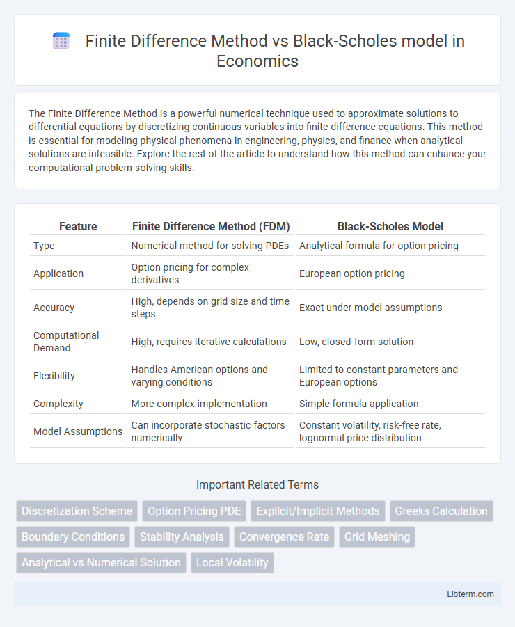
| Feature | Finite Difference Method (FDM) | Black-Scholes Model |
|---|---|---|
| Type | Numerical method for solving PDEs | Analytical formula for option pricing |
| Application | Option pricing for complex derivatives | European option pricing |
| Accuracy | High, depends on grid size and time steps | Exact under model assumptions |
| Computational Demand | High, requires iterative calculations | Low, closed-form solution |
| Flexibility | Handles American options and varying conditions | Limited to constant parameters and European options |
| Complexity | More complex implementation | Simple formula application |
| Model Assumptions | Can incorporate stochastic factors numerically | Constant volatility, risk-free rate, lognormal price distribution |
Introduction to Option Pricing Models
Finite Difference Method (FDM) and Black-Scholes model are fundamental tools in option pricing theory, offering distinct approaches to valuing derivatives. The Black-Scholes model provides a closed-form analytical solution for European options by assuming constant volatility and a lognormal price distribution. In contrast, the Finite Difference Method numerically solves the partial differential equations governing option prices, allowing for greater flexibility in handling complex boundary conditions and American-style options.
Overview of the Black-Scholes Model
The Black-Scholes model is a mathematical framework used to price European-style options by solving a partial differential equation based on stochastic processes and volatility assumptions. It assumes constant volatility and risk-free interest rates, leading to a closed-form analytical solution for option prices. This model is fundamental in financial engineering and derivatives trading, providing a benchmark for option valuation compared to numerical methods like the Finite Difference Method.
Fundamentals of the Finite Difference Method
The Finite Difference Method (FDM) approximates solutions to differential equations by discretizing continuous variables into a grid, enabling numerical computation of option prices. It relies on replacing derivatives in the Black-Scholes partial differential equation with finite difference quotients, effectively transforming the problem into a system of algebraic equations. FDM offers flexibility in handling complex boundary conditions and can accommodate American options by incorporating early exercise features through iterative algorithms.
Assumptions in Black-Scholes vs. Finite Difference
The Black-Scholes model assumes constant volatility, continuous trading, and a lognormal distribution of asset prices, relying on closed-form solutions for option pricing. In contrast, the Finite Difference Method (FDM) does not impose strict assumptions about volatility or market conditions, instead numerically solving partial differential equations under more flexible and realistic settings. FDM's adaptability allows it to handle complex boundary conditions and variable parameters that the Black-Scholes model cannot easily accommodate.
Mathematical Formulation: Black-Scholes Model
The Black-Scholes model is based on a partial differential equation derived from the geometric Brownian motion assumption for asset prices, defined as V/t + (1/2)s2S22V/S2 + rSV/S - rV = 0. This equation represents the price evolution of European-style options, where V is the option price, S is the underlying asset price, s is volatility, r is the risk-free interest rate, and t is time. The model's closed-form analytical solution provides explicit pricing formulas, contrasting the numerical approximation approach used in the finite difference method.
Mathematical Formulation: Finite Difference Schemes
Finite Difference Method (FDM) employs discrete grid points to approximate derivatives in the Black-Scholes Partial Differential Equation, converting it into a system of algebraic equations for numerical solution. Explicit, implicit, and Crank-Nicolson schemes are common finite difference techniques, balancing between computational stability and accuracy in option pricing. These schemes handle boundary conditions and time-stepping to model option values effectively under various market scenarios.
Computational Efficiency and Implementation
The Finite Difference Method offers greater flexibility in handling complex boundary conditions and American-style options but typically requires extensive computational time due to grid discretization and iterative solvers. The Black-Scholes model provides closed-form solutions for European options, enabling rapid computation with less implementation complexity, yet lacks adaptability for path-dependent or early-exercise features. Optimizing the Finite Difference Method through advanced numerical techniques can improve efficiency but still generally demands higher resource usage compared to the straightforward Black-Scholes formula.
Flexibility for Complex Financial Derivatives
The Finite Difference Method offers greater flexibility for pricing complex financial derivatives by numerically solving partial differential equations under various boundary conditions and payoff structures. In contrast, the Black-Scholes model provides closed-form solutions primarily for European-style options with simpler assumptions such as constant volatility and risk-free rates. This adaptability makes the Finite Difference Method more suitable for derivatives with path-dependent features, early exercise options, and varying market parameters.
Accuracy and Stability Considerations
The Finite Difference Method offers flexible grid discretization, enhancing accuracy in pricing complex derivative structures with boundary conditions, but may require fine mesh and small time steps for stability, increasing computational cost. The Black-Scholes model provides closed-form solutions for European options, ensuring high efficiency and stability but assumes constant volatility and risk-free rates, limiting accuracy for instruments with stochastic features. Stability in finite difference schemes depends on the chosen numerical method (explicit, implicit, or Crank-Nicolson), with implicit and Crank-Nicolson methods generally providing better stability and convergence compared to the explicit scheme.
Practical Applications and Use Cases
The Finite Difference Method is widely used for numerically solving partial differential equations in option pricing, particularly for American options where early exercise features complicate analytic solutions. The Black-Scholes model provides closed-form solutions for European options, offering quick and straightforward pricing under assumptions of constant volatility and risk-free rates. In practical applications, Finite Difference excels in handling complex derivatives with boundary conditions and varying parameters, while Black-Scholes remains preferred for standard option valuation due to its computational efficiency and ease of use.
Finite Difference Method Infographic