The Ordered Probit model is a statistical technique used for analyzing ordinal dependent variables where outcomes have a natural order but unknown intervals. It estimates the probability of each ordered category by modeling a latent continuous variable underlying the observed outcomes. Explore the article to understand how the Ordered Probit model can enhance your data analysis and decision-making processes.
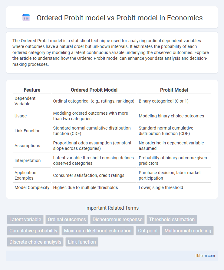
Table of Comparison
| Feature | Ordered Probit Model | Probit Model |
|---|---|---|
| Dependent Variable | Ordinal categorical (e.g., ratings, rankings) | Binary categorical (0 or 1) |
| Usage | Modeling ordered outcomes with more than two categories | Modeling binary choice outcomes |
| Link Function | Standard normal cumulative distribution function (CDF) | Standard normal cumulative distribution function (CDF) |
| Assumptions | Proportional odds assumption (constant slope across categories) | No ordering in dependent variable assumed |
| Interpretation | Latent variable threshold crossing defines observed categories | Probability of binary outcome given predictors |
| Application Examples | Consumer satisfaction, credit ratings | Purchase decision, labor market participation |
| Model Complexity | Higher, due to multiple thresholds | Lower, single threshold |
Introduction to Probit and Ordered Probit Models
The Probit model is a statistical technique used for binary dependent variables, estimating the probability that an outcome belongs to one of two categories based on predictor variables. The Ordered Probit model extends this framework to handle ordinal dependent variables with more than two categories, preserving the natural order without assuming equal distances between them. Both models rely on the cumulative normal distribution function to link linear predictors to probabilities, making them essential tools in fields like economics, social sciences, and medical research for categorical data analysis.
Understanding the Probit Model
The Probit model estimates binary outcome probabilities by modeling the latent variable using the cumulative normal distribution, making it ideal for dichotomous dependent variables. The Ordered Probit model extends this approach to ordinal dependent variables with more than two ordered categories, capturing the probability of outcomes falling within specific thresholds. Both models assume a latent continuous variable underlying observed categorical outcomes but differ in handling the ordinal structure inherent in ordered responses.
Exploring the Ordered Probit Model
The Ordered Probit model extends the Probit model by accommodating dependent variables with ordinal outcomes, allowing for more nuanced analysis of ranked categories rather than binary responses. It estimates the probability that an observation falls into a specific ordered category based on a latent continuous variable partitioned by threshold parameters. This model is essential in fields like economics and social sciences where responses represent ordered choices, enhancing interpretability and predictive accuracy over the standard Probit model.
Key Differences Between Probit and Ordered Probit Models
The Probit model is used for binary dependent variables, estimating the probability of two mutually exclusive outcomes based on the cumulative normal distribution. The Ordered Probit model extends this framework to handle ordinal dependent variables with more than two ordered categories by modeling threshold parameters that separate these categories. Key differences include the nature of the dependent variable--binary for Probit versus ordinal for Ordered Probit--and the complexity of interpretation, where Ordered Probit coefficients relate to latent variables and category thresholds rather than direct probabilities.
Data Types Suitable for Each Model
The Ordered Probit model is specifically designed for ordinal dependent variables where the outcome categories have a natural order but unknown interval distances, such as survey responses ranging from "strongly disagree" to "strongly agree." In contrast, the Probit model is suitable for binary dependent variables with only two categories, like success/failure or yes/no outcomes, where the response is dichotomous without an inherent order. Selecting the appropriate model depends on the nature of the dependent variable: ordered discrete data fits Ordered Probit, while binary outcomes are analyzed using the standard Probit model.
Assumptions Underlying Both Models
The Ordered Probit model assumes the dependent variable is ordinal with a natural order, capturing latent continuous tendencies segmented by threshold parameters, while the Probit model treats the dependent variable as binary, reflecting two distinct outcome categories. Both models assume a normally distributed error term and independent observations to produce consistent estimates. Key differences hinge on how the latent variable translates into observed responses: the Ordered Probit partitions outcomes into multiple ordered categories, whereas the Probit model dichotomizes the latent variable into a single binary result.
Estimation Procedures and Techniques
The Ordered Probit model estimates latent ordinal dependent variables by maximizing the likelihood function with threshold parameters delimiting outcome categories, often employing numerical optimization techniques such as Newton-Raphson or BFGS algorithms. In contrast, the standard Probit model estimates binary outcomes using maximum likelihood estimation but without threshold parameters, simplifying the likelihood function to a single cutoff point. Both models rely on iterative procedures, yet the Ordered Probit requires joint estimation of regression coefficients and cut-points, increasing computational complexity compared to the binary Probit model.
Interpretation of Model Results
The Ordered Probit model extends the Probit model by handling ordinal dependent variables with more than two categories, allowing for the estimation of threshold parameters that separate outcome categories. Interpretation of coefficients in the Ordered Probit model involves understanding their impact on the latent variable and the probability of the dependent variable falling into specific ordered categories, rather than direct changes in probabilities as in the binary Probit model. Marginal effects are crucial in both models, but in the Ordered Probit, they must be calculated for each category to interpret the influence of explanatory variables on the likelihood of different ordered outcomes.
Applications and Use Cases
The Ordered Probit model is specifically designed for analyzing ordinal dependent variables, making it ideal for applications involving rating scales, survey responses with ordered categories, and customer satisfaction levels. In contrast, the Probit model is suited for binary outcome variables, such as yes/no decisions, medical diagnoses, or credit approval processes. Businesses and researchers use Ordered Probit models to capture the inherent order in multi-level categorical data, while the Probit model is preferred for straightforward classification tasks with two possible outcomes.
Choosing the Right Model for Your Analysis
The Ordered Probit model is ideal for analyzing ordinal dependent variables where categories have a meaningful order but no fixed interval, such as customer satisfaction ratings. The standard Probit model suits binary outcomes, efficiently estimating the probability of a single event occurrence, like purchase or non-purchase decisions. Selecting between these models depends on the data structure: use Ordered Probit for ordered categorical data and Probit for binary classification tasks to maximize analytical accuracy and interpretability.
Ordered Probit model Infographic