Time-varying state refers to dynamic systems where the state variables evolve over time due to changes in inputs or environmental conditions. Understanding these variations is crucial for designing effective control strategies and predicting system behavior accurately. Explore the rest of the article to deepen your understanding of time-varying states and their applications.
Table of Comparison
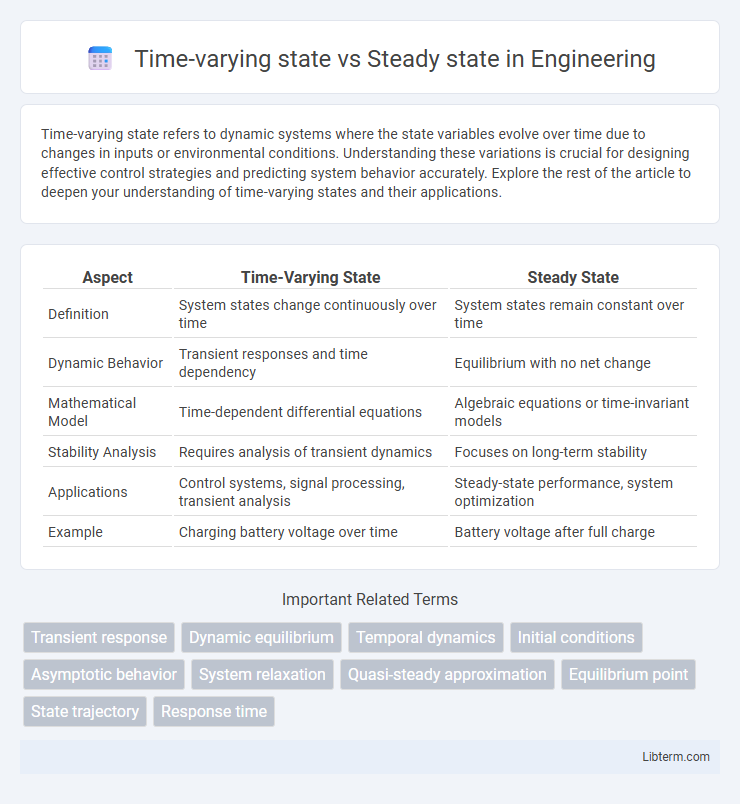
| Aspect | Time-Varying State | Steady State |
|---|---|---|
| Definition | System states change continuously over time | System states remain constant over time |
| Dynamic Behavior | Transient responses and time dependency | Equilibrium with no net change |
| Mathematical Model | Time-dependent differential equations | Algebraic equations or time-invariant models |
| Stability Analysis | Requires analysis of transient dynamics | Focuses on long-term stability |
| Applications | Control systems, signal processing, transient analysis | Steady-state performance, system optimization |
| Example | Charging battery voltage over time | Battery voltage after full charge |
Introduction to Time-Varying State and Steady State
Time-varying state refers to system conditions that change over time, influenced by dynamic inputs and transient responses, whereas steady state describes a condition where system variables remain constant despite continuous operation. In control theory and signal processing, understanding time-varying states is crucial for analyzing transient behaviors, while steady-state analysis simplifies system behavior by focusing on long-term equilibrium. Differentiating these states enables accurate modeling and prediction of system performance in engineering and physics applications.
Defining Time-Varying State
Time-varying state refers to dynamic system conditions that change over time, contrasting with steady state where variables remain constant. It involves analyzing transient behaviors and system responses to fluctuations in inputs or environmental factors. Understanding time-varying states is crucial for modeling real-world processes like electrical circuits, chemical reactions, and control systems where conditions evolve continuously.
Understanding Steady State
Steady state refers to a condition in dynamic systems where variables remain constant over time despite ongoing processes, indicating equilibrium between inputs and outputs. Understanding steady state involves analyzing system behavior once transient effects have diminished, allowing prediction of long-term performance and stability. This concept is crucial in fields like control engineering, thermodynamics, and economics for modeling processes and designing systems that maintain consistent operation.
Key Differences Between Time-Varying and Steady States
Time-varying states involve dynamic changes in system variables over time, reflecting transient responses and evolving conditions, while steady states represent equilibrium conditions where variables remain constant. In control systems and signal processing, time-varying states are characterized by variable system parameters and non-static outputs, whereas steady states imply stability and time-invariant behavior. The key differences lie in temporal variability, system stability, and response predictability, critical for applications in engineering, physics, and economics.
Mathematical Representation of Time-Varying State
Time-varying state in mathematical systems is represented by differential or difference equations that describe how state variables change over time, typically expressed as \( \dot{x}(t) = A(t)x(t) + B(t)u(t) \) for continuous systems or \( x_{k+1} = A_k x_k + B_k u_k \) for discrete systems. The state transition matrix \( \Phi(t, t_0) \) plays a crucial role in capturing the system's evolution from an initial state \( x(t_0) \) to \( x(t) \) in time-varying systems. This contrasts with steady-state, where \( \dot{x}(t) = 0 \) and the system variables remain constant, typically solved by setting \( Ax + Bu = 0 \) in a time-invariant context.
Mathematical Representation of Steady State
Steady state in mathematical modeling is represented by setting the time derivatives of system variables to zero, implying no change over time and allowing simplification of differential equations into algebraic equations. This representation facilitates solving for equilibrium points where the system's variables remain constant. In contrast, time-varying states involve differential equations with non-zero derivatives that describe dynamic changes in state variables over time.
Applications of Time-Varying State in Engineering and Science
Time-varying state analysis is crucial in engineering and science for modeling dynamic systems like control systems, signal processing, and climate models, where system properties change over time. These applications rely on time-dependent variables to predict system behavior, optimize performance, and design adaptive algorithms in fields such as robotics, electrical circuits, and environmental monitoring. The ability to capture transient responses and evolutions in time-varying states enables more accurate simulation and real-time decision-making compared to steady-state assumptions.
Applications of Steady State in Real-World Systems
Steady state conditions are pivotal in engineering systems such as electrical circuits, where constant current and voltage levels enable reliable operation and performance analysis. In chemical process industries, maintaining steady state allows for optimized reactor function and consistent product quality by ensuring stable temperature and concentration levels. Mechanical systems like rotating machinery rely on steady state operation to minimize wear and enhance efficiency through uniform speed and load conditions.
Advantages and Limitations of Each State
Time-varying state models capture dynamic system behaviors and transient responses, providing detailed insights into processes that change over time, which is advantageous for real-time monitoring and control but often requires complex computations and extensive data. Steady state models simplify analysis by assuming system variables remain constant over time, offering ease of calculation and faster results, yet they may overlook crucial fluctuations and transient phenomena critical for accurate system understanding. Choosing between time-varying and steady state approaches depends on the balance between the need for precision and computational efficiency in applications like chemical engineering, control systems, and environmental modeling.
Summary and Future Perspectives
Time-varying state analysis captures dynamic system behaviors and transient responses crucial for real-time control and adaptive processes, contrasting with steady-state analysis that focuses on long-term equilibrium conditions and system stability. Emerging computational methods and machine learning techniques enhance the accuracy and speed of time-varying state estimation, offering improved predictive capabilities for complex systems. Future perspectives emphasize integrating real-time data analytics and hybrid modeling approaches to optimize system performance and resilience across diverse engineering and scientific applications.
Time-varying state Infographic