The steady-state response of a system describes its behavior after transient effects have settled, reflecting how it reacts to continuous inputs over time. Understanding this response is crucial for predicting long-term system performance and ensuring stability in control systems. Explore the rest of the article to learn how to analyze and apply steady-state response concepts effectively.
Table of Comparison
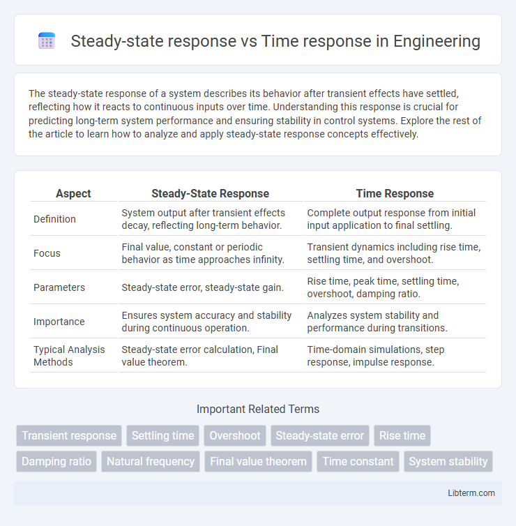
| Aspect | Steady-State Response | Time Response |
|---|---|---|
| Definition | System output after transient effects decay, reflecting long-term behavior. | Complete output response from initial input application to final settling. |
| Focus | Final value, constant or periodic behavior as time approaches infinity. | Transient dynamics including rise time, settling time, and overshoot. |
| Parameters | Steady-state error, steady-state gain. | Rise time, peak time, settling time, overshoot, damping ratio. |
| Importance | Ensures system accuracy and stability during continuous operation. | Analyzes system stability and performance during transitions. |
| Typical Analysis Methods | Steady-state error calculation, Final value theorem. | Time-domain simulations, step response, impulse response. |
Introduction to System Responses
System responses describe how dynamic systems react to inputs over time, with the steady-state response representing the long-term behavior after transient effects diminish. The time response encompasses the entire output from initial input application, including both transient and steady-state phases. Analyzing steady-state and time responses is essential for understanding system stability, performance, and predicting output behavior under various conditions.
Defining Steady-State Response
Steady-state response is the behavior of a system output after transient effects have decayed and the system reaches equilibrium under a constant input. It reflects the final output value or periodic behavior when the system stabilizes over time. Time response includes both the transient response, showing how the system reacts initially, and the steady-state response, which indicates long-term system performance.
Understanding Time Response
Time response in control systems characterizes how a system's output evolves over time following an input or disturbance, emphasizing transient behavior such as rise time, settling time, and overshoot. Understanding time response is crucial for evaluating system stability and performance before the output reaches a steady-state. Analyzing time response provides insight into system dynamics, ensuring efficient control design and optimal transient performance.
Key Differences Between Steady-State and Time Response
Steady-state response refers to the behavior of a system after transient effects have dissipated, reflecting its long-term output under constant input conditions. Time response encompasses the entire system reaction from the initial input application to the point where steady-state is reached, including transient and steady-state phases. Key differences lie in their analysis focus; steady-state response emphasizes output stability and final value, while time response evaluates dynamic characteristics such as rise time, settling time, and transient oscillations.
Mathematical Representation of Responses
Steady-state response is mathematically represented by the particular solution of a system's differential equation when the input is sinusoidal, typically expressed as a phasor or sinusoidal function in the form \( A \sin(\omega t + \phi) \), where \( A \) is amplitude, \( \omega \) is angular frequency, and \( \phi \) is phase shift. Time response encompasses the total solution, combining the homogeneous (transient) solution and the particular (steady-state) solution, usually represented as \( x(t) = x_h(t) + x_p(t) \), where \( x_h(t) \) includes exponential decaying terms and \( x_p(t) \) reflects the steady-state sinusoidal response. These mathematical forms allow precise analysis of systems in both transient and long-term operation scenarios using Laplace transforms and complex frequency domain techniques.
Importance in Control Systems
Steady-state response reflects the long-term behavior of a control system when it reaches equilibrium, providing crucial information about system accuracy and error margins. Time response characterizes how quickly and effectively the system reacts to changes or disturbances, indicating stability and transient performance. Understanding both responses is essential for designing control systems that achieve desired performance criteria, ensuring reliability and precision in real-world applications.
Factors Affecting Steady-State and Time Response
Steady-state response is primarily influenced by system parameters such as gain, damping ratio, and natural frequency, which determine the final output magnitude and stability after transient effects subside. Time response depends on factors like initial conditions, input type, system order, and the presence of poles or zeros, affecting how quickly and smoothly the system reaches steady state. Understanding these factors allows for precise control over transient overshoot, settling time, rise time, and steady-state error in control system design.
Common Applications in Engineering
Steady-state response analysis plays a crucial role in control systems engineering for predicting system behavior under constant inputs, ensuring stability and desired output accuracy in applications like motor speed control and power regulation. Time response evaluation is essential in signal processing and mechanical systems for assessing transient behaviors such as damping, overshoot, and settling time, which are critical in automotive suspension design and robotics. Both responses are integral in aerospace engineering for fine-tuning flight control systems and in electrical circuit design to optimize filters and amplifiers for performance under varying conditions.
Advantages and Limitations
Steady-state response provides valuable information about a system's behavior under constant input, offering a clear understanding of long-term output performance and stability. Time response captures the dynamic characteristics, including rise time, settling time, and transient behavior, crucial for evaluating system reaction to sudden changes or disturbances. While steady-state analysis lacks insight into transient dynamics, time response evaluation may be computationally intensive and sensitive to noise or modeling inaccuracies.
Conclusion and Future Trends
Steady-state response analysis provides crucial insights into the long-term behavior of dynamic systems, highlighting system stability and performance under constant inputs, while time response focuses on transient behavior, revealing how systems react to changes over time. Advances in machine learning and adaptive control algorithms promise enhanced accuracy in predicting both steady-state and transient responses, enabling more robust and efficient system designs. Future trends point towards integrated frameworks combining real-time data analytics with traditional control theory to optimize dynamic system performance across diverse applications.
Steady-state response Infographic