Gegenbauer polynomials are a class of orthogonal polynomials that generalize Legendre and Chebyshev polynomials, playing a crucial role in approximation theory and solutions to differential equations. These polynomials are essential in problems involving spherical harmonics and appear frequently in mathematical physics, especially in quantum mechanics and potential theory. Explore the rest of the article to understand how Gegenbauer polynomials can enhance your understanding of advanced mathematical concepts and applications.
Table of Comparison
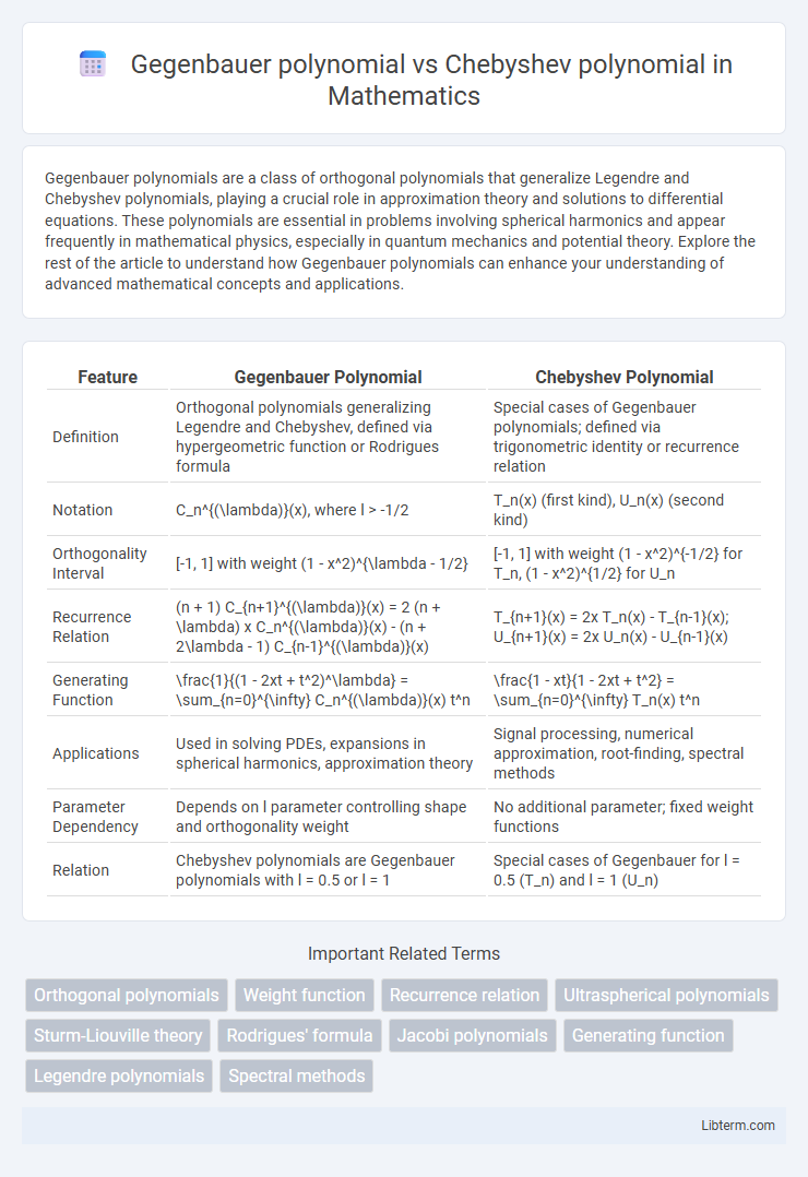
| Feature | Gegenbauer Polynomial | Chebyshev Polynomial |
|---|---|---|
| Definition | Orthogonal polynomials generalizing Legendre and Chebyshev, defined via hypergeometric function or Rodrigues formula | Special cases of Gegenbauer polynomials; defined via trigonometric identity or recurrence relation |
| Notation | C_n^{(\lambda)}(x), where l > -1/2 | T_n(x) (first kind), U_n(x) (second kind) |
| Orthogonality Interval | [-1, 1] with weight (1 - x^2)^{\lambda - 1/2} | [-1, 1] with weight (1 - x^2)^{-1/2} for T_n, (1 - x^2)^{1/2} for U_n |
| Recurrence Relation | (n + 1) C_{n+1}^{(\lambda)}(x) = 2 (n + \lambda) x C_n^{(\lambda)}(x) - (n + 2\lambda - 1) C_{n-1}^{(\lambda)}(x) | T_{n+1}(x) = 2x T_n(x) - T_{n-1}(x); U_{n+1}(x) = 2x U_n(x) - U_{n-1}(x) |
| Generating Function | \frac{1}{(1 - 2xt + t^2)^\lambda} = \sum_{n=0}^{\infty} C_n^{(\lambda)}(x) t^n | \frac{1 - xt}{1 - 2xt + t^2} = \sum_{n=0}^{\infty} T_n(x) t^n |
| Applications | Used in solving PDEs, expansions in spherical harmonics, approximation theory | Signal processing, numerical approximation, root-finding, spectral methods |
| Parameter Dependency | Depends on l parameter controlling shape and orthogonality weight | No additional parameter; fixed weight functions |
| Relation | Chebyshev polynomials are Gegenbauer polynomials with l = 0.5 or l = 1 | Special cases of Gegenbauer for l = 0.5 (T_n) and l = 1 (U_n) |
Introduction to Orthogonal Polynomials
Gegenbauer polynomials, generalizing Legendre and Chebyshev polynomials, form an important class of orthogonal polynomials defined on the interval [-1, 1] with respect to the weight function (1 - x^2)^(l - 1/2), where l > -1/2. Chebyshev polynomials, a special case of Gegenbauer polynomials with l = 0 or 1, exhibit orthogonality under specific weight functions and are widely used in approximation theory and numerical analysis. Both polynomial families serve as foundational tools in solving problems related to Fourier expansions, spectral methods, and mathematical physics due to their orthogonality properties and recurrence relations.
Defining Gegenbauer Polynomials
Gegenbauer polynomials, also known as ultraspherical polynomials, generalize Chebyshev polynomials by introducing a parameter l that controls their weighting function and orthogonality on the interval [-1, 1]. Defined via the hypergeometric function or the Rodrigues formula, Gegenbauer polynomials satisfy the differential equation \((1-x^2)y'' - (2\lambda+1)xy' + n(n+2\lambda)y = 0\). While Chebyshev polynomials of the first and second kind are special cases of Gegenbauer polynomials with l = 0.5 and l = 1 respectively, Gegenbauer polynomials provide a broader framework for expansions in weighted L2 spaces.
Overview of Chebyshev Polynomials
Chebyshev polynomials, defined on the interval [-1, 1], are a sequence of orthogonal polynomials widely used in approximation theory and numerical analysis due to their minimax property and efficient calculation via recurrence relations. These polynomials, especially of the first kind (T_n), minimize the maximum error in polynomial interpolation, making them crucial for spectral methods and solving differential equations. Gegenbauer polynomials generalize Chebyshev polynomials by introducing a parameter that controls the polynomial family's weight function and orthogonality properties, extending their applicability in higher-dimensional problems.
Mathematical Formulations and Recurrence Relations
Gegenbauer polynomials \(C_n^{(\lambda)}(x)\) generalize Legendre and Chebyshev polynomials and are defined by the hypergeometric series or Rodrigues' formula, satisfying the differential equation \((1 - x^2) y'' - (2\lambda + 1) x y' + n(n + 2\lambda) y = 0\). Chebyshev polynomials of the first kind \(T_n(x)\) and second kind \(U_n(x)\) are special cases of Gegenbauer polynomials corresponding to \(\lambda = 0.5\) and \(\lambda = 1\) respectively, with explicit forms \(T_n(x) = \cos(n \arccos x)\) and \(U_n(x) = \frac{\sin((n+1) \arccos x)}{\sin(\arccos x)}\). The recurrence relations for Gegenbauer polynomials are \((n+1) C_{n+1}^{(\lambda)}(x) = 2 (n+\lambda) x C_n^{(\lambda)}(x) - (n + 2 \lambda -1) C_{n-1}^{(\lambda)}(x)\), while Chebyshev polynomials satisfy simpler recurrences: \(T_{n+1}(x) = 2x T_n(x) - T_{n-1}(x)\) and \(U_{n+1}(x) = 2x U_n(x) - U_{n-1}(x)\).
Weight Functions and Orthogonality Properties
Gegenbauer polynomials \(C_n^{(\lambda)}(x)\) are orthogonal with respect to the weight function \((1 - x^2)^{\lambda - \frac{1}{2}}\) on the interval \([-1,1]\), where \(\lambda > -\frac{1}{2}\). Chebyshev polynomials of the first kind \(T_n(x)\) correspond to the special case \(\lambda = 0\) in the Gegenbauer family, with the weight function \(\frac{1}{\sqrt{1 - x^2}}\), while Chebyshev polynomials of the second kind \(U_n(x)\) correspond to \(\lambda = 1\) with weight \(\sqrt{1 - x^2}\). Both systems exhibit orthogonality on \([-1,1]\) under their respective weights, making Gegenbauer polynomials a generalization of Chebyshev polynomials and providing a broader framework for handling singular weight functions in approximation theory.
Special Cases and Interconnections
Gegenbauer polynomials generalize Chebyshev polynomials as special cases when the parameter l equals 0.5 or 1, corresponding to Chebyshev polynomials of the first and second kinds, respectively. These interconnections highlight the hierarchical structure among classical orthogonal polynomials and provide a unified framework for approximation theory and spectral methods.
Applications in Numerical Analysis
Gegenbauer polynomials are widely used in numerical analysis for solving differential equations and spectral methods due to their orthogonality properties on the interval [-1, 1] with a weight function, enhancing convergence in approximations. Chebyshev polynomials, particularly of the first kind, are pivotal in polynomial interpolation and minimax approximation, minimizing the maximum error and improving numerical stability in algorithms. Both polynomials serve as basis functions in spectral methods, but Gegenbauer polynomials offer more flexibility in handling singularities, while Chebyshev polynomials excel in fast transform computations like the Fast Fourier Transform (FFT).
Properties: Zeros and Extremal Values
Gegenbauer polynomials have zeros that are all real, simple, and lie within the interval (-1, 1), with their distribution dependent on the parameter a, influencing orthogonality and weight functions. Chebyshev polynomials, a special case of Gegenbauer polynomials with a = 0.5, possess zeros explicitly given by cos((2k-1)p/(2n)) for k=1,...,n, providing extremal values of +-1 that equioscillate on [-1, 1]. Both polynomial families serve crucial roles in approximation theory, where the location of zeros and extremal properties enable optimal interpolation and minimization of errors in numerical analysis.
Computational Advantages and Limitations
Gegenbauer polynomials generalize Chebyshev polynomials, allowing more flexible parameter tuning for improved numerical stability in higher-dimensional problems, but this flexibility increases computational complexity compared to the simpler recurrence relations of Chebyshev polynomials. Chebyshev polynomials benefit from efficient algorithms like the Fast Fourier Transform (FFT) for spectral methods and exhibit near-minimal polynomial interpolation error, making them computationally advantageous in 1D approximation tasks. However, Gegenbauer polynomials require more computational resources for evaluation and integration due to their parameter-dependent nature, limiting their practicality in large-scale or real-time computations.
Summary: Choosing Between Gegenbauer and Chebyshev Polynomials
Gegenbauer polynomials generalize Chebyshev polynomials and are more flexible for solving differential equations with varying parameters due to their dependence on an additional parameter, l. Chebyshev polynomials, a special case of Gegenbauer polynomials, are computationally efficient and widely used in numerical approximation, interpolation, and spectral methods. Selecting between them depends on the problem's specific symmetry properties and weight functions, with Gegenbauer favored for more general orthogonal expansions and Chebyshev preferred for simpler, fast-converging approximations.
Gegenbauer polynomial Infographic