Laplace transform converts complex time-domain functions into simpler s-domain expressions, facilitating easier analysis of electrical circuits, control systems, and differential equations. This powerful mathematical tool simplifies solving linear ordinary differential equations by transforming derivatives into algebraic terms. Explore the rest of the article to deepen your understanding of how Laplace transform can enhance your problem-solving skills.
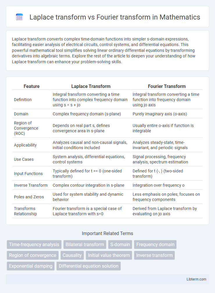
Table of Comparison
| Feature | Laplace Transform | Fourier Transform |
|---|---|---|
| Definition | Integral transform converting a time function into complex frequency domain using s = s + jo | Integral transform converting a time function into frequency domain using jo axis |
| Domain | Complex frequency domain (s-plane) | Purely imaginary axis (o-axis) |
| Region of Convergence (ROC) | Depends on real part s, defines convergence area in s-plane | Usually entire o-axis if function is integrable |
| Applicability | Analyzes causal and non-causal signals, initial conditions included | Analyzes steady-state, time-invariant, and periodic signals |
| Use Cases | System analysis, differential equations, control systems | Signal processing, frequency analysis, spectrum estimation |
| Input Functions | Typically defined for t >= 0 (one-sided transform) | Defined for t (-, ) (two-sided transform) |
| Inverse Transform | Complex contour integration in s-plane | Integration over frequency o |
| Poles and Zeros | Used for system stability and dynamic behavior | Less emphasis on poles; focuses on frequency components |
| Transforms Relationship | Fourier transform is a special case of Laplace transform with s=0 | Derived from Laplace transform by evaluating on jo axis |
Introduction to Laplace and Fourier Transforms
The Laplace transform converts a time-domain function into a complex frequency-domain representation, primarily used for analyzing linear time-invariant systems and solving differential equations with initial conditions. The Fourier transform decomposes a signal into its constituent sinusoidal frequencies, providing a frequency-spectrum representation essential for signal processing and frequency analysis. Both transforms enable system behavior characterization, yet the Laplace transform incorporates exponential decay enabling handling of unstable or transient systems, while the Fourier transform assumes signals are stable and periodic or extend infinitely in time.
Historical Background and Development
The Laplace transform, developed by Pierre-Simon Laplace in the 18th century, originated from probability theory and celestial mechanics, offering a method to simplify differential equations by transforming functions into complex frequency domains. The Fourier transform, introduced by Joseph Fourier in the early 19th century, emerged from studies on heat conduction, representing functions as sums of sinusoidal components to analyze frequency spectra. Both transforms revolutionized mathematical physics and engineering, with the Laplace transform focusing on unilateral, complex-variable analysis and the Fourier transform excelling in bilateral, periodic signal decomposition.
Mathematical Definitions and Formulations
The Laplace transform is defined as \( \mathcal{L}\{f(t)\} = \int_0^\infty e^{-st} f(t) \, dt \), where \( s \) is a complex number, allowing analysis of functions with exponential growth or decay. The Fourier transform is given by \( \mathcal{F}\{f(t)\} = \int_{-\infty}^\infty e^{-i\omega t} f(t) \, dt \), utilizing purely imaginary complex frequency \( i\omega \) to decompose signals into sinusoidal components. Both transforms convert time-domain functions into complex frequency-domain representations but differ in integral limits and the nature of their complex frequency variables.
Core Principles: Time-Domain vs Frequency-Domain
The Laplace transform converts a time-domain signal into a complex frequency-domain representation, providing insights into system stability and transient behavior through the s-plane. The Fourier transform maps a time-domain signal strictly into the frequency domain using real frequencies, revealing the signal's spectral content and steady-state characteristics. While the Laplace transform handles exponential growth and decay, the Fourier transform assumes signal stationarity and is primarily used for analyzing periodic or steady-state signals.
Regions of Convergence and Applicability
The Laplace transform features a complex variable \(s = \sigma + j\omega\) with a defined Region of Convergence (ROC) that determines the existence and stability of the transform, making it suitable for analyzing causal and non-causal signals in control systems and differential equations. The Fourier transform is a special case of the Laplace transform evaluated along the imaginary axis (\(s = j\omega\)), with a ROC that must include this axis for the transform to exist, primarily applied to steady-state and periodic signals in frequency analysis. Understanding the ROC is crucial for choosing the appropriate transform: Laplace transform offers greater flexibility for transient analysis, while Fourier transform excels in frequency domain representation of signals with infinite energy or steady-state behavior.
Main Use Cases: Engineering and Science Applications
Laplace transform is primarily used in engineering for analyzing and solving linear time-invariant systems, control theory, and differential equations, especially where initial conditions and system stability are critical. Fourier transform excels in signal processing, frequency analysis, image processing, and communications by decomposing signals into their frequency components, facilitating filtering and spectral analysis. Both transforms are essential tools in physics and electrical engineering for modeling dynamic systems and studying wave behavior.
Advantages and Limitations of Each Transform
The Laplace transform excels in analyzing systems with initial conditions and handling exponential growth or decay in signals, making it ideal for stability and control system design; however, it requires complex contour integration and may be less intuitive for frequency domain analysis. The Fourier transform provides comprehensive frequency spectrum analysis for steady-state signals and is computationally efficient due to Fast Fourier Transform algorithms, but it assumes signal periodicity or infinite duration, limiting its application in transient or non-stationary signal analysis. Both transforms serve critical roles in engineering and physics, yet selecting between them depends on the nature of the signal and the specific requirements of time or frequency domain analysis.
Laplace Transform vs Fourier Transform: Key Differences
The Laplace transform is used primarily for analyzing linear time-invariant systems with initial conditions, transforming functions from the time domain to the complex frequency domain (s-plane), while the Fourier transform converts signals to the frequency domain (jo-axis) assuming signals are stable and extend infinitely. Unlike the Fourier transform, the Laplace transform can handle exponentially growing signals and provides information about system stability and transient behavior through its complex frequency parameter. The Laplace transform's region of convergence distinguishes it from the Fourier transform, which requires functions to be absolutely integrable for convergence.
Conversion and Relationship Between the Two
The Laplace transform generalizes the Fourier transform by incorporating a complex frequency variable s = s + jo, allowing analysis of both transient and steady-state behaviors through integration of a function multiplied by e^(-st). The Fourier transform emerges as a special case of the Laplace transform when the real part s equals zero, simplifying to integration with e^(-jot) and focusing on frequency domain representation. These transforms are interconnected tools in signal processing and systems analysis, where the Laplace transform offers convergence advantages and the Fourier transform facilitates spectral decomposition.
Conclusion and Practical Recommendations
The Laplace transform excels in analyzing systems with initial conditions and transient behaviors, making it ideal for control engineering and differential equation solutions. The Fourier transform is best suited for steady-state signal analysis and frequency domain representation, often used in signal processing and communications. For practical applications, choose the Laplace transform when dealing with time-dependent system dynamics and the Fourier transform for frequency spectrum analysis of periodic or aperiodic signals.
Laplace transform Infographic