Gegenbauer polynomials are a class of orthogonal polynomials that generalize Legendre and Chebyshev polynomials, playing a significant role in mathematical analysis and approximation theory. They are widely used in solving differential equations, quantum mechanics, and expanding functions in higher-dimensional spaces. Discover how Gegenbauer polynomials can enhance your understanding of advanced mathematical concepts by reading the full article.
Table of Comparison
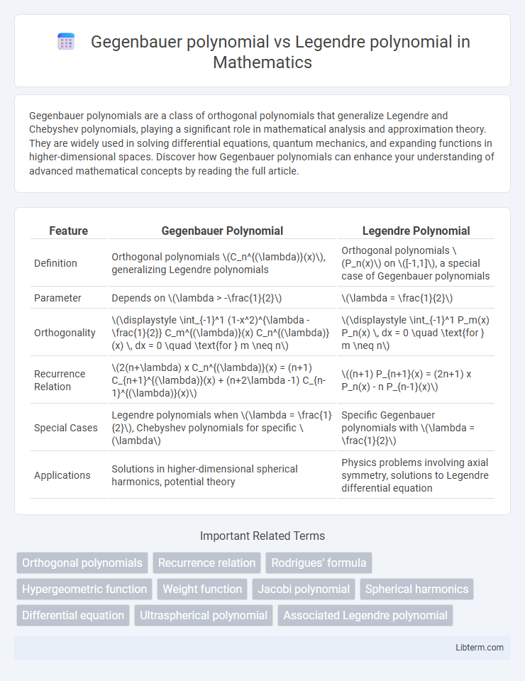
| Feature | Gegenbauer Polynomial | Legendre Polynomial |
|---|---|---|
| Definition | Orthogonal polynomials \(C_n^{(\lambda)}(x)\), generalizing Legendre polynomials | Orthogonal polynomials \(P_n(x)\) on \([-1,1]\), a special case of Gegenbauer polynomials |
| Parameter | Depends on \(\lambda > -\frac{1}{2}\) | \(\lambda = \frac{1}{2}\) |
| Orthogonality | \(\displaystyle \int_{-1}^1 (1-x^2)^{\lambda - \frac{1}{2}} C_m^{(\lambda)}(x) C_n^{(\lambda)}(x) \, dx = 0 \quad \text{for } m \neq n\) | \(\displaystyle \int_{-1}^1 P_m(x) P_n(x) \, dx = 0 \quad \text{for } m \neq n\) |
| Recurrence Relation | \(2(n+\lambda) x C_n^{(\lambda)}(x) = (n+1) C_{n+1}^{(\lambda)}(x) + (n+2\lambda -1) C_{n-1}^{(\lambda)}(x)\) | \((n+1) P_{n+1}(x) = (2n+1) x P_n(x) - n P_{n-1}(x)\) |
| Special Cases | Legendre polynomials when \(\lambda = \frac{1}{2}\), Chebyshev polynomials for specific \(\lambda\) | Specific Gegenbauer polynomials with \(\lambda = \frac{1}{2}\) |
| Applications | Solutions in higher-dimensional spherical harmonics, potential theory | Physics problems involving axial symmetry, solutions to Legendre differential equation |
Introduction to Orthogonal Polynomials
Gegenbauer polynomials, also known as ultraspherical polynomials, generalize Legendre polynomials by incorporating an additional parameter \(\lambda\), which adjusts their weight function and orthogonality interval. Both are members of the classical orthogonal polynomials family, with Legendre polynomials arising as a special case of Gegenbauer polynomials when \(\lambda = \frac{1}{2}\). These polynomials are widely used in solving problems in mathematical physics, particularly in expansions of functions on spherical domains and in spectral methods for differential equations.
Defining Gegenbauer and Legendre Polynomials
Gegenbauer polynomials \(C_n^{(\lambda)}(x)\) generalize Legendre polynomials by incorporating a parameter \(\lambda > -\frac{1}{2}\), defined via the generating function \((1 - 2xt + t^2)^{-\lambda} = \sum_{n=0}^\infty C_n^{(\lambda)}(x) t^n\). Legendre polynomials \(P_n(x)\) emerge as a special case of Gegenbauer polynomials with \(\lambda = \frac{1}{2}\), satisfying the Legendre differential equation \(\frac{d}{dx}[(1-x^2)\frac{d}{dx}P_n(x)] + n(n+1)P_n(x) = 0\). Both sets form orthogonal polynomials on the interval \([-1, 1]\), with \(\{P_n(x)\}\) playing a pivotal role in solving physics problems involving spherical symmetry.
Historical Background and Development
Gegenbauer polynomials, introduced by Leopold Gegenbauer in the late 19th century, generalized Legendre polynomials by extending the orthogonal polynomial family associated with hypergeometric functions. Legendre polynomials, developed earlier by Adrien-Marie Legendre in the 18th century, originated in solving problems of celestial mechanics and potential theory. Both polynomial families play fundamental roles in mathematical physics, with Gegenbauer polynomials providing a broader framework that includes Legendre polynomials as a special case when their parameter equals 0.5.
Mathematical Formulation and Recurrence Relations
Gegenbauer polynomials, denoted as \(C_n^{(\lambda)}(x)\), generalize Legendre polynomials \(P_n(x)\) by introducing a parameter \(\lambda\), with the relation \(P_n(x) = C_n^{(1/2)}(x)\). Their mathematical formulation is given by the Rodrigues' formula: \(C_n^{(\lambda)}(x) = \frac{(-2)^n \Gamma(n+\lambda) }{n! \Gamma(\lambda)} (1 - x^2)^{-\lambda + \frac{1}{2}} \frac{d^n}{dx^n} \left( (1-x^2)^{n+\lambda - \frac{1}{2}} \right)\). The recurrence relations for Gegenbauer polynomials are expressed as \(2x(n+\lambda) C_n^{(\lambda)}(x) = (n+1) C_{n+1}^{(\lambda)}(x) + (n+2\lambda -1) C_{n-1}^{(\lambda)}(x)\), while Legendre polynomials satisfy \( (n+1) P_{n+1}(x) = (2n+1) x P_n(x) - n P_{n-1}(x) \), highlighting their specific recursion without the parameter \(\lambda\).
Orthogonality Properties Compared
Gegenbauer polynomials \( C_n^{(\lambda)}(x) \) are orthogonal on the interval \([-1, 1]\) with respect to the weight function \((1 - x^2)^{\lambda - \frac{1}{2}}\), where \(\lambda > -\frac{1}{2}\), providing a generalization of Legendre polynomials. Legendre polynomials \( P_n(x) \) form a special case of Gegenbauer polynomials with \(\lambda = \frac{1}{2}\), orthogonal under the uniform weight function \(w(x) = 1\) on \([-1, 1]\). The choice of weight functions impacts the inner product space, making Gegenbauer polynomials applicable for diverse spectral methods and spherical harmonics expansions, while Legendre polynomials excel in problems requiring simpler orthogonality conditions.
Parameter Differences and Special Cases
Gegenbauer polynomials C_n^(l)(x) generalize Legendre polynomials P_n(x) by introducing the parameter l, where Legendre polynomials correspond to the special case l = 1/2. The parameter l in Gegenbauer polynomials controls weighting and orthogonality over the interval [-1,1] with respect to the weight function (1 - x2)^(l - 1/2), whereas Legendre polynomials are orthogonal with uniform weighting (l = 1/2). This parameter difference allows Gegenbauer polynomials to encompass a broader class of orthogonal polynomials applicable in higher dimensions and more general spherical harmonics expansions.
Weight Functions and Interval of Orthogonality
Gegenbauer polynomials are orthogonal on the interval [-1, 1] with respect to the weight function (1 - x^2)^(l - 1/2), where l > -1/2, generalizing Legendre polynomials which correspond to the special case l = 1/2. Legendre polynomials are also orthogonal on [-1, 1], but with a constant weight function of 1, indicating uniform weight across the interval. The differing weight functions impact their applications in solving differential equations and expansions in series where the underlying symmetry and boundary conditions vary.
Applications in Physics and Engineering
Gegenbauer polynomials generalize Legendre polynomials and are extensively utilized in solving higher-dimensional Laplace equations, making them essential in quantum mechanics and electromagnetism for representing spherical harmonics in multi-dimensional spaces. Legendre polynomials primarily appear in classical physics problems involving spherical symmetry such as gravitational and electrostatic potential calculations, and are the basis of expansions in problems governed by Laplace's equation in three dimensions. Both polynomial families play critical roles in numerical methods like spectral methods for differential equations, with Gegenbauer polynomials offering enhanced flexibility for anisotropic and higher-dimensional problems in engineering simulations.
Relationship and Transformations Between Polynomials
Gegenbauer polynomials \( C_n^{(\lambda)}(x) \) generalize Legendre polynomials \( P_n(x) \), with the latter being a special case for \(\lambda = \frac{1}{2}\). Transformations between these polynomials involve expressing Legendre polynomials as Gegenbauer polynomials using the relation \( P_n(x) = C_n^{(1/2)}(x) \). The orthogonality properties and recurrence relations of Gegenbauer polynomials extend those of Legendre polynomials, facilitating expansions in higher-dimensional spherical harmonics.
Summary: Choosing Between Gegenbauer and Legendre
Gegenbauer polynomials generalize Legendre polynomials and are preferred when working with higher-dimensional hyperspherical harmonics due to their additional parameter allowing better flexibility in fitting complex functions. Legendre polynomials are a special case of Gegenbauer polynomials with parameter a=1/2, making them ideal for problems with spherical symmetry in three dimensions and simpler computational applications. Selecting between these depends on the dimensional context and the desired balance between computational complexity and approximation accuracy.
Gegenbauer polynomial Infographic