Brownian motion describes the random movement of particles suspended in a fluid resulting from their collision with fast-moving molecules. This phenomenon explains diffusion processes fundamental to various scientific fields, including physics, chemistry, and biology. Explore the article further to understand how Brownian motion impacts your view of molecular interactions and stochastic processes.
Table of Comparison
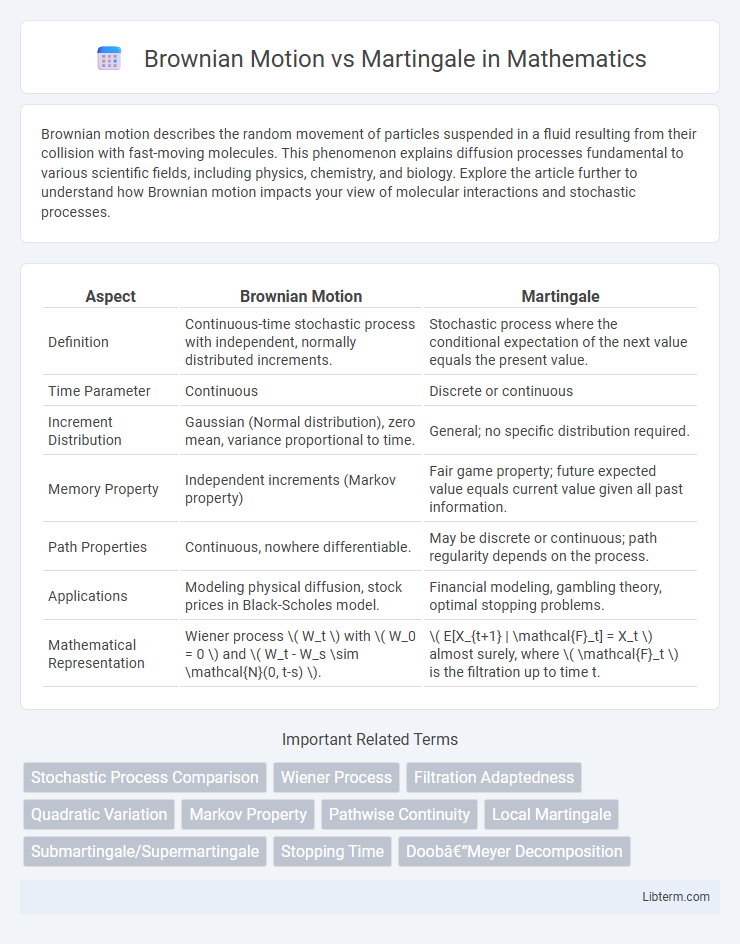
| Aspect | Brownian Motion | Martingale |
|---|---|---|
| Definition | Continuous-time stochastic process with independent, normally distributed increments. | Stochastic process where the conditional expectation of the next value equals the present value. |
| Time Parameter | Continuous | Discrete or continuous |
| Increment Distribution | Gaussian (Normal distribution), zero mean, variance proportional to time. | General; no specific distribution required. |
| Memory Property | Independent increments (Markov property) | Fair game property; future expected value equals current value given all past information. |
| Path Properties | Continuous, nowhere differentiable. | May be discrete or continuous; path regularity depends on the process. |
| Applications | Modeling physical diffusion, stock prices in Black-Scholes model. | Financial modeling, gambling theory, optimal stopping problems. |
| Mathematical Representation | Wiener process \( W_t \) with \( W_0 = 0 \) and \( W_t - W_s \sim \mathcal{N}(0, t-s) \). | \( E[X_{t+1} | \mathcal{F}_t] = X_t \) almost surely, where \( \mathcal{F}_t \) is the filtration up to time t. |
Introduction to Brownian Motion and Martingale
Brownian Motion, a continuous-time stochastic process characterized by independent, normally distributed increments, serves as a fundamental model for random movement in fields such as physics and finance. Martingale, a stochastic process with the property that its conditional expected future value equals its current value, represents a fair game in probability theory and is pivotal in financial modeling for pricing derivatives. Understanding Brownian Motion lays the groundwork for grasping martingale theory, as Brownian Motion itself is a martingale under standard filtration with zero drift.
Mathematical Foundations
Brownian motion is a continuous-time stochastic process characterized by independent, normally distributed increments and almost surely continuous paths, forming the basis of diffusion models in probability theory. In contrast, a martingale is a stochastic process where the conditional expectation of the next value, given the past, equals the present value, ensuring no predictable drift and encapsulating the concept of a "fair game." While Brownian motion serves as a prototypical example of a martingale with Gaussian increments, martingales encompass a broader class of processes pivotal in proving fundamental theorems such as the optional stopping theorem and in financial modeling through martingale measures.
Key Properties of Brownian Motion
Brownian motion features continuous paths, stationary and independent increments, and normally distributed changes with mean zero and variance proportional to time. It exhibits the Markov property, meaning its future evolution depends only on the present state, not on the past trajectory. Martingales generalize the fair game property, ensuring conditional expected values remain constant over time, but Brownian motion specifically models random diffusion with Gaussian increments and continuous, almost surely nowhere differentiable paths.
Key Properties of Martingales
Martingales are stochastic processes characterized by the property that their expected future value, conditional on the present and past values, equals the current value, demonstrating a "fair game" condition without drift. Unlike Brownian motion, which is continuous with independent Gaussian increments, martingales emphasize conditional expectation and the preservation of the process's current value as its best predictor. Key properties of martingales include the martingale property itself, the optional stopping theorem, and uniform integrability, which together facilitate advanced probabilistic modeling in finance and stochastic calculus.
Differences in Stochastic Processes
Brownian motion is a continuous-time stochastic process characterized by independent, normally distributed increments and almost surely continuous paths, representing random fluctuations in physical systems. Martingales, on the other hand, are stochastic processes where the conditional expectation of the future value, given all past information, equals the present value, emphasizing a "fair game" property without necessarily requiring continuous paths or Gaussian increments. Unlike Brownian motion, which has specific distributional properties and continuous trajectories, martingales encompass a broader class of processes that may be discrete or continuous and are primarily defined by their conditional expectation structure.
Brownian Motion as a Martingale
Brownian motion, a continuous-time stochastic process with independent, normally distributed increments, is a classic example of a martingale due to its property of having zero conditional drift and finite variance. This martingale characteristic ensures that the expected future value of Brownian motion, given all prior information, equals its current value, making it a fundamental model in mathematical finance and stochastic calculus. The martingale property of Brownian motion underpins its use in option pricing models like Black-Scholes and in various filtering and prediction algorithms.
Applications in Finance and Physics
Brownian motion serves as the foundation for modeling stochastic processes in physics, describing the random movement of particles in fluids, while in finance, it underpins the Black-Scholes option pricing model by capturing asset price fluctuations. Martingales are central to financial mathematics in representing "fair game" price processes to ensure no arbitrage opportunities, enabling risk-neutral valuation and derivative pricing. In physics, martingale concepts assist in analyzing the fairness and predictability of stochastic systems, complementing Brownian motion in understanding random dynamics.
Simulation Techniques
Simulating Brownian motion involves generating continuous-time stochastic processes with independent, normally distributed increments, typically using the Euler-Maruyama method or the Wiener process approximation. Martingale simulation often leverages discrete-time models, such as random walks or conditional expectation-based updates, ensuring that the expected future value equals the current state. Advanced simulation techniques incorporate variance reduction methods like antithetic variates and control variates to enhance efficiency and accuracy in both Brownian motion and martingale models.
Common Misconceptions
Brownian motion and martingales are often confused, but they differ fundamentally in their mathematical properties and applications; Brownian motion exhibits continuous paths with independent increments, while martingales emphasize conditional expectation without drift. A common misconception is that all martingales are Brownian motions, though martingales can include discrete-time processes and need not have Gaussian increments or continuous paths. Understanding that Brownian motion is a specific example of a martingale with continuous time and normally distributed increments clarifies their distinct roles in stochastic calculus and financial modeling.
Conclusion and Future Perspectives
Brownian motion and martingale processes both serve as fundamental models in stochastic analysis, with Brownian motion characterized by continuous paths and Gaussian increments, while martingales emphasize the conditional expectation property. Their distinctions underpin various applications in finance, physics, and mathematics, especially in option pricing and risk assessment. Future research is likely to explore hybrid models integrating Brownian paths with martingale structures to enhance predictive accuracy and robustness in complex dynamic systems.
Brownian Motion Infographic