Maintaining a balanced lifestyle is essential for optimal health and well-being. Proper nutrition, regular exercise, and adequate sleep contribute significantly to your overall energy levels and mental clarity. Discover practical tips and strategies in the rest of the article to help you achieve a healthier, more balanced life.
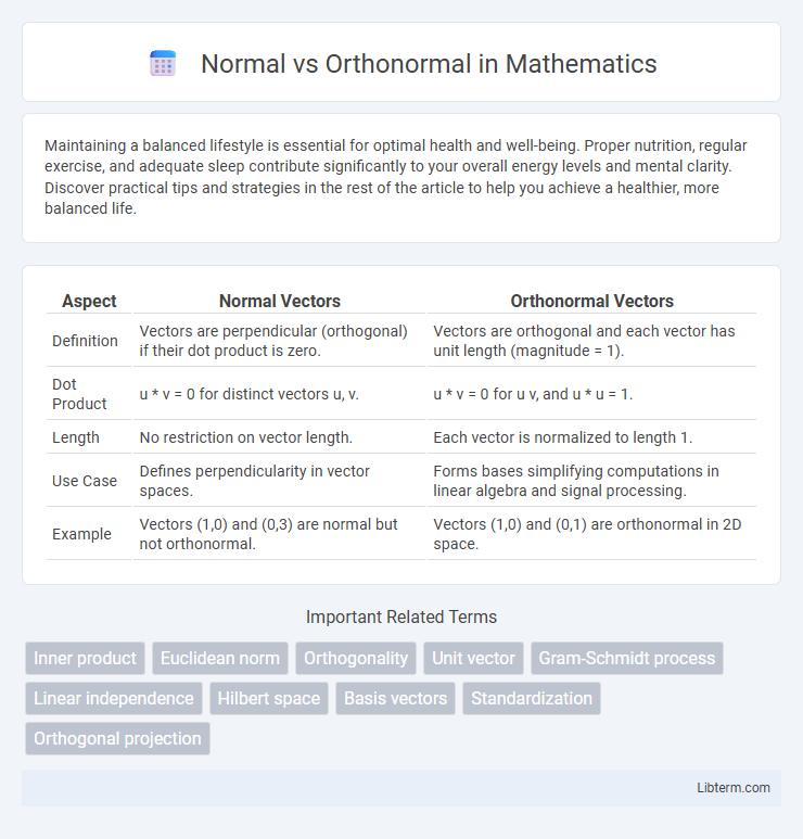
Table of Comparison
| Aspect | Normal Vectors | Orthonormal Vectors |
|---|---|---|
| Definition | Vectors are perpendicular (orthogonal) if their dot product is zero. | Vectors are orthogonal and each vector has unit length (magnitude = 1). |
| Dot Product | u * v = 0 for distinct vectors u, v. | u * v = 0 for u v, and u * u = 1. |
| Length | No restriction on vector length. | Each vector is normalized to length 1. |
| Use Case | Defines perpendicularity in vector spaces. | Forms bases simplifying computations in linear algebra and signal processing. |
| Example | Vectors (1,0) and (0,3) are normal but not orthonormal. | Vectors (1,0) and (0,1) are orthonormal in 2D space. |
Understanding Vectors: Normal vs Orthonormal
Normal vectors have a magnitude that can vary and are orthogonal to a surface or plane, essential in geometry and physics for defining directions and orientations. Orthonormal vectors are not only orthogonal but also normalized to a unit length, forming a basis that simplifies computations in linear algebra and computer graphics. Understanding these distinctions aids in vector space analysis, where orthonormal sets ensure independence and stability in transformations.
Defining Normal Vectors
Normal vectors are defined as vectors perpendicular to a surface or plane, characterized by their direction without a fixed magnitude. Orthonormal vectors not only maintain this perpendicularity but also have unit length, ensuring both direction and scale are standardized. These orthonormal vectors form the basis for coordinate systems, facilitating precise computations in geometry and linear algebra.
What Makes a Set Orthonormal?
A set is orthonormal when each vector in the set has a unit norm and is mutually orthogonal to all other vectors, ensuring their dot products equal zero. Normalization scales vectors to have length one, while orthogonality guarantees perpendicularity among vectors, combining to form an orthonormal set. This property is fundamental in linear algebra for simplifying vector space representations and facilitating computations in fields such as quantum mechanics and signal processing.
Key Differences: Normal and Orthonormal
Normal vectors have a magnitude that can vary, whereas orthonormal vectors have a magnitude exactly equal to one. Normal vectors are not necessarily perpendicular, but orthonormal vectors are always mutually perpendicular and normalized. The key difference lies in orthonormality combining both orthogonality and unit length, ensuring both direction and scale are standardized.
Importance in Linear Algebra
Normal matrices, characterized by commuting with their conjugate transpose, enable diagonalization through unitary transformations, simplifying complex linear algebra problems. Orthonormal sets, featuring mutually perpendicular vectors with unit length, provide a stable and efficient basis for vector spaces, essential for preserving lengths and angles during transformations. The interplay between normal and orthonormal structures is crucial for optimizing matrix computations, spectral analysis, and maintaining numerical stability in algorithms.
Mathematical Representation and Notation
Normal vectors are simply vectors in a vector space with no specific length requirement, typically denoted as v or \(\mathbf{v}\), while orthonormal vectors are a set of vectors that are both orthogonal (perpendicular) and normalized to unit length, represented as \(\mathbf{u}_i\) where \(\|\mathbf{u}_i\| = 1\) and \(\mathbf{u}_i \cdot \mathbf{u}_j = 0\) for \(i \neq j\). The mathematical notation for a normal vector \(\mathbf{v}\) involves its components or magnitude \(\|\mathbf{v}\|\), whereas an orthonormal basis \(\{\mathbf{u}_1, \mathbf{u}_2, ..., \mathbf{u}_n\}\) satisfies the Kronecker delta condition \(\mathbf{u}_i \cdot \mathbf{u}_j = \delta_{ij}\). Orthonormality is crucial in simplifying matrix representations and transformations since the inner product structure preserves lengths and angles by definition.
Practical Applications in Computing
Normal vectors simplify geometric computations by ensuring perpendicularity without scale constraints, essential in graphics rendering and collision detection algorithms. Orthonormal sets extend this by combining perpendicularity with unit length, optimizing matrix operations like rotations and transformations in computer vision and robotics. Utilizing orthonormal bases improves numerical stability and efficiency in algorithms such as QR decomposition and Fourier transforms, crucial for signal processing and machine learning.
Methods for Obtaining Orthonormal Sets
Methods for obtaining orthonormal sets primarily involve the Gram-Schmidt process, which orthogonalizes a given set of vectors and then normalizes each vector to unit length. Another approach includes the use of QR decomposition, where a matrix is factored into an orthonormal matrix Q and an upper triangular matrix R, ensuring the columns of Q form an orthonormal basis. These techniques guarantee orthonormal sets crucial for simplifying computations in linear algebra, signal processing, and quantum mechanics.
Normalization and Orthogonalization Explained
Normalization involves scaling vectors to have a unit norm, ensuring each vector's length is one, which is essential for creating orthonormal sets. Orthogonalization refers to the process of converting a set of vectors into mutually perpendicular vectors, where their dot products are zero, thus achieving orthogonality. Combining both processes produces an orthonormal set, where vectors are both orthogonal and normalized, widely used in linear algebra, signal processing, and machine learning for simplifying computations and enhancing numerical stability.
Summary Table: Normal vs Orthonormal Properties
A normal matrix commutes with its conjugate transpose, satisfying the equation A*A = AA*, whereas an orthonormal matrix is a special type of normal matrix with orthonormal columns and rows, meaning Q*Q = QQ* = I. Normal matrices can be unitarily diagonalized, maintaining eigenvector orthogonality, while orthonormal matrices preserve vector norms and angles, ensuring length and direction remain unchanged. The summary table highlights key differences: normal matrices include symmetric, skew-symmetric, and unitary matrices, whereas orthonormal matrices are strictly unitary with columns forming an orthonormal basis.
Normal Infographic