Elliptic offers advanced blockchain analytics and fraud detection solutions designed to help businesses and financial institutions identify illicit activities and ensure regulatory compliance. Their cutting-edge technology leverages machine learning and extensive data sets to provide deep insights into cryptocurrency transactions. Explore the rest of the article to discover how Elliptic can protect your assets and enhance your security measures.
Table of Comparison
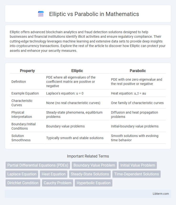
| Property | Elliptic | Parabolic |
|---|---|---|
| Definition | PDE where all eigenvalues of the coefficient matrix are positive or negative | PDE with one zero eigenvalue and the rest positive or negative |
| Example Equation | Laplace's equation: u = 0 | Heat equation: u_t = au |
| Characteristic Curves | None (no real characteristic curves) | One family of characteristic curves |
| Physical Interpretation | Steady-state phenomena, equilibrium problems | Diffusion and heat propagation problems |
| Boundary/Initial Conditions | Boundary value problems | Initial-boundary value problems |
| Solution Smoothness | Typically smooth and stable solutions | Smooth solutions with evolving time behavior |
Introduction to Elliptic and Parabolic Equations
Elliptic equations, such as Laplace's and Poisson's equations, model steady-state phenomena with boundary value problems characterized by smooth, continuous solutions. Parabolic equations, exemplified by the heat equation, describe time-dependent processes involving diffusion or heat transfer, capturing how states evolve over time with initial and boundary conditions. Both equation types are fundamental in partial differential equations, representing distinct physical processes with unique mathematical properties and solution techniques.
Defining Elliptic Partial Differential Equations
Elliptic partial differential equations (PDEs) are characterized by the positive definiteness of their coefficient matrix, ensuring smooth and stable solutions often modeling steady-state phenomena like heat distribution or electrostatics. Unlike parabolic PDEs, which describe time-dependent processes such as diffusion, elliptic PDEs do not involve temporal derivatives and represent equilibrium conditions. The canonical example of an elliptic PDE is Laplace's equation, 2u = 0, highlighting the role of elliptic operators in boundary value problems with well-posedness and unique solutions under appropriate conditions.
Understanding Parabolic Partial Differential Equations
Parabolic partial differential equations, such as the heat equation, model time-dependent processes where diffusion or heat flow occurs, characterized by their first-order time derivative and second-order spatial derivatives. These equations exhibit smoothing properties, meaning initial irregularities in the solution tend to dissipate over time, reflecting the physical behavior of heat conduction and diffusion. Unlike elliptic equations, which describe steady-state scenarios, parabolic PDEs require initial conditions and often boundary conditions to ensure well-posedness and uniqueness of solutions.
Key Mathematical Differences: Elliptic vs Parabolic
Elliptic partial differential equations, such as Laplace's equation, feature no real characteristic curves, implying that solutions are generally smooth and well-behaved across the domain. Parabolic partial differential equations, exemplified by the heat equation, involve a single family of real characteristic curves, reflecting time-dependent diffusion processes with directional smoothing effects. Elliptic equations often represent steady-state phenomena, while parabolic equations model transient, time-evolving systems.
Physical and Engineering Applications
Elliptic partial differential equations commonly describe steady-state phenomena such as electrostatics, heat distribution, and incompressible fluid flow, where solutions are smooth and boundary conditions dictate the entire domain. Parabolic equations model time-dependent processes including heat conduction and diffusion, capturing transient behavior with solutions evolving over time toward equilibrium. Engineering applications leverage elliptic equations for designing stable structures and steady-state thermal systems, while parabolic equations are crucial for simulating transient thermal analysis and pollutant dispersion in fluids.
Boundary and Initial Conditions Explained
Elliptic partial differential equations, such as Laplace's equation, require boundary conditions specified on the entire boundary of the spatial domain, with no initial conditions involved because they describe steady-state systems. Parabolic partial differential equations, exemplified by the heat equation, need initial conditions representing the starting state of the system and boundary conditions defined on the spatial boundary that evolve over time. The key distinction lies in elliptic problems emphasizing spatial boundary conditions alone, while parabolic problems combine temporal initial conditions with spatial boundary constraints to capture dynamic behavior.
Solution Methods and Techniques
Elliptic partial differential equations typically require iterative methods such as the Gauss-Seidel or Multigrid techniques to achieve convergence to steady-state solutions, relying on boundary conditions throughout the domain. Parabolic equations often employ time-stepping methods like the Crank-Nicolson or implicit Euler schemes, which balance stability and accuracy for evolving solutions over time. Finite difference, finite element, and finite volume methods are commonly adapted to both elliptic and parabolic problems, optimizing spatial discretization based on the problem's geometry and solution smoothness.
Stability and Behavior of Solutions
Elliptic equations, such as Laplace's equation, typically exhibit stable solutions characterized by smooth and bounded behavior, reflecting equilibrium states in physical systems. Parabolic equations, exemplified by the heat equation, describe time-dependent processes with solutions that evolve smoothly over time, demonstrating both stability and smoothing effects as they approach steady states. The fundamental difference lies in elliptic equations modeling spatial phenomena with inherent stability, while parabolic equations capture dynamic temporal evolution with dissipative properties.
Real-world Examples and Use Cases
Elliptic partial differential equations model steady-state phenomena such as heat distribution in a metal plate or electrostatic potential in a capacitor, reflecting equilibrium conditions. Parabolic partial differential equations describe time-dependent processes like heat conduction in a rod and option pricing in financial markets, capturing evolution over time. Real-world applications of elliptic equations include structural engineering and steady-state fluid flow, while parabolic equations are crucial in thermodynamics and diffusion processes in environmental science.
Summary: Choosing Between Elliptic and Parabolic Models
Elliptic models are best suited for steady-state problems where the solution is smooth and boundary conditions are well-defined, commonly used in heat conduction and electrostatics. Parabolic models effectively describe time-dependent processes such as diffusion and heat transfer, capturing the evolution of systems over time. Selecting between elliptic and parabolic models depends on whether the problem requires a time-independent solution or dynamic analysis of transient phenomena.
Elliptic Infographic