Hyperbolic language exaggerates statements to create a strong emotional impact or emphasize a point, often used in literature, advertising, and everyday speech. Understanding hyperbolic expressions helps you discern between literal and figurative meanings, enhancing your communication skills and critical thinking. Explore the rest of the article to discover how hyperbole shapes language and influences perception.
Table of Comparison
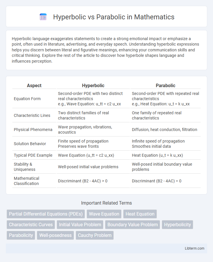
| Aspect | Hyperbolic | Parabolic |
|---|---|---|
| Equation Form | Second-order PDE with two distinct real characteristics e.g., Wave Equation: u_tt = c2 u_xx |
Second-order PDE with repeated real characteristics e.g., Heat Equation: u_t = k u_xx |
| Characteristic Lines | Two distinct families of real characteristics | One family of repeated real characteristics |
| Physical Phenomena | Wave propagation, vibrations, acoustics | Diffusion, heat conduction, filtration |
| Solution Behavior | Finite speed of propagation Preserves wave fronts |
Infinite speed of propagation Smoothes initial data |
| Typical PDE Example | Wave Equation (u_tt = c2 u_xx) | Heat Equation (u_t = k u_xx) |
| Stability & Uniqueness | Well-posed initial value problems | Well-posed initial boundary value problems |
| Mathematical Classification | Discriminant (B2 - 4AC) > 0 | Discriminant (B2 - 4AC) = 0 |
Introduction to Hyperbolic and Parabolic Equations
Hyperbolic and parabolic equations are fundamental types of partial differential equations (PDEs) used to describe different physical phenomena. Hyperbolic equations model wave propagation and dynamic systems with finite speed of signal transmission, exemplified by the classic wave equation. Parabolic equations characterize diffusion processes and heat conduction with infinite speed of propagation, with the heat equation as a primary example.
Fundamental Differences: Hyperbolic vs Parabolic
Hyperbolic and parabolic equations differ fundamentally in their mathematical structure and physical interpretations. Hyperbolic equations model wave propagation and signal transmission, characterized by real and distinct eigenvalues indicating time-dependent, oscillatory solutions. Parabolic equations describe diffusion processes, featuring a single repeated eigenvalue leading to smooth, dissipative behavior over time.
Mathematical Definitions and Properties
Hyperbolic equations describe phenomena with wave-like solutions and are characterized by real and distinct eigenvalues, ensuring well-posed initial value problems with finite propagation speeds. Parabolic equations involve diffusion-like processes, exhibiting a single repeated eigenvalue that leads to smoothing effects over time and infinite propagation speeds in idealized scenarios. Both equation types are second-order partial differential equations but differ fundamentally in their characteristic forms and the nature of their solutions.
Physical Phenomena Modeled
Hyperbolic equations typically model wave propagation and dynamic systems with finite speed signals, such as sound waves, electromagnetic waves, and fluid flow problems like shock waves. Parabolic equations describe diffusion-like processes where effects spread gradually over time, including heat conduction, chemical diffusion, and price evolution in financial markets. Understanding the distinction aids in selecting appropriate mathematical tools for accurately simulating physical phenomena governed by either rapid or gradual changes.
Examples in Engineering and Physics
Hyperbolic equations describe wave propagation and heat conduction phenomena, such as the wave equation governing vibrations in strings or electromagnetic waves in transmission lines. Parabolic equations model diffusion processes and steady-state heat distribution, exemplified by the heat equation used in thermal analysis of materials and semiconductor devices. Engineering applications of hyperbolic equations include stress waves in solids and signal processing, while parabolic equations are essential for modeling pollutant dispersion in air and groundwater flow.
Key Solution Techniques
Hyperbolic partial differential equations are primarily solved using characteristic methods that trace wave propagation paths, while parabolic equations often rely on techniques like finite difference methods and implicit time-stepping to handle diffusion processes. The method of characteristics efficiently handles hyperbolic equations by converting PDEs into ordinary differential equations along characteristic curves. Parabolic equations are commonly approached using Crank-Nicolson or backward Euler schemes for stability in time-dependent solutions involving heat conduction or diffusion phenomena.
Boundary and Initial Conditions
Hyperbolic partial differential equations require both initial and boundary conditions to uniquely determine the solution, often modeling wave propagation where initial displacement and velocity are specified along with boundary constraints. Parabolic equations, such as the heat equation, primarily depend on initial conditions with boundary conditions shaping the solution over time, emphasizing diffusion processes. The well-posedness of hyperbolic problems hinges on initial values specified on a time slice and boundary values on spatial boundaries, while parabolic problems typically need initial temperature distribution and boundary temperature or flux specifications.
Stability and Uniqueness of Solutions
Hyperbolic partial differential equations, such as the wave equation, exhibit well-posedness characterized by unique solutions that are stable under small perturbations in initial data, ensuring predictable evolution of wave propagation. Parabolic equations, like the heat equation, guarantee uniqueness and stability of solutions with smoothing effects over time, which lead to gradual dissipation of initial irregularities. Stability in hyperbolic equations is often associated with finite speed of propagation, while parabolic equations feature infinite speed of propagation, influencing their respective solution behaviors and physical interpretations.
Applications and Real-world Implications
Hyperbolic equations model wave propagation and signal transmission in mediums like acoustics, electromagnetics, and fluid dynamics, making them crucial in designing communication systems and earthquake analysis. Parabolic equations describe diffusion processes, heat conduction, and pricing in financial mathematics, enabling accurate forecasting and risk management. The distinct mathematical behavior of hyperbolic versus parabolic models directly influences algorithm selection and solution stability in engineering and scientific simulations.
Summary and Future Directions
Hyperbolic systems, characterized by wave propagation and finite speed signals, contrast with parabolic systems, which model diffusion processes with infinite speed propagation. Research in hyperbolic equations emphasizes improving numerical methods for stability and accuracy, while parabolic studies focus on enhanced modeling of heat and mass transfer phenomena. Future directions include developing hybrid models that integrate hyperbolic and parabolic behaviors to better simulate complex real-world systems in engineering and physics.
Hyperbolic Infographic