The finite difference method is a numerical technique used to approximate solutions to differential equations by replacing derivatives with finite difference quotients. It converts continuous problems into discrete ones, enabling computational analysis of heat transfer, fluid dynamics, and other physical phenomena. Explore the rest of the article to understand how this method can enhance your approach to solving complex equations.
Table of Comparison
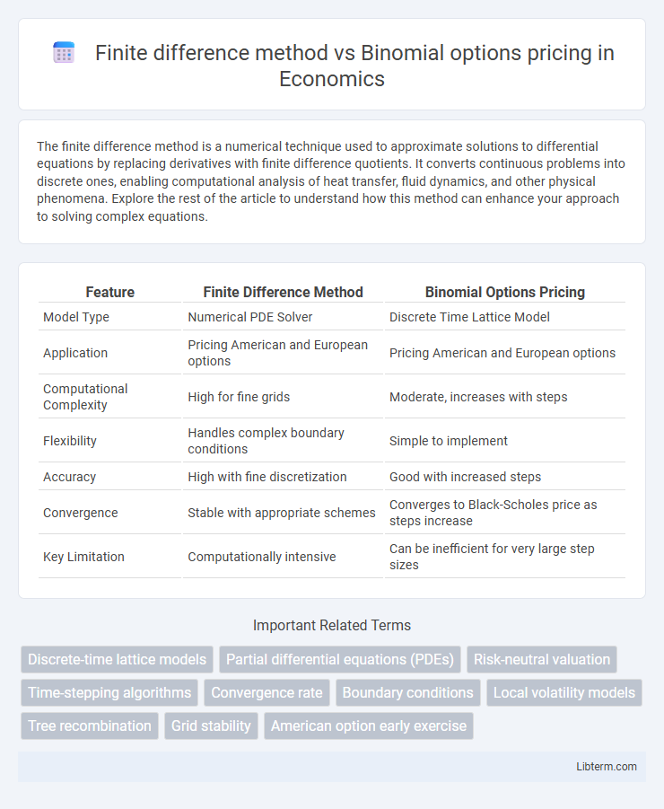
| Feature | Finite Difference Method | Binomial Options Pricing |
|---|---|---|
| Model Type | Numerical PDE Solver | Discrete Time Lattice Model |
| Application | Pricing American and European options | Pricing American and European options |
| Computational Complexity | High for fine grids | Moderate, increases with steps |
| Flexibility | Handles complex boundary conditions | Simple to implement |
| Accuracy | High with fine discretization | Good with increased steps |
| Convergence | Stable with appropriate schemes | Converges to Black-Scholes price as steps increase |
| Key Limitation | Computationally intensive | Can be inefficient for very large step sizes |
Introduction to Option Pricing Methods
Finite difference methods use partial differential equations to numerically solve the Black-Scholes equation, providing flexibility in modeling complex option features such as American exercise and barriers. Binomial options pricing employs a discrete-time lattice model to approximate potential future asset prices, allowing intuitive handling of early exercise and path-dependent options. Both approaches offer distinct computational techniques crucial for valuing a wide range of financial derivatives under various market conditions.
Overview of the Binomial Options Pricing Model
The Binomial Options Pricing Model uses a discrete-time framework to model the possible future price movements of an underlying asset, allowing for flexible handling of American-style options due to its ability to incorporate early exercise features. It constructs a recombining price tree where each node represents possible asset prices at a given point in time, facilitating step-by-step calculation of option value through backward induction. This method contrasts with the Finite Difference Method, which solves the Black-Scholes partial differential equation numerically but may be less intuitive for handling early exercise and path-dependent options.
Fundamentals of the Finite Difference Method
The Finite Difference Method (FDM) approximates partial differential equations like the Black-Scholes equation by discretizing time and asset price into a grid, allowing numerical option pricing. It solves for option values at each node using difference equations, providing flexibility in handling complex boundary conditions and American-style options. Compared to the Binomial Option Pricing Model, which simulates price movements through a recombining tree, FDM offers higher accuracy and stability for multidimensional problems but requires more computational effort.
Mathematical Foundations: Binomial vs Finite Difference
The finite difference method relies on discretizing the partial differential equations governing option prices, such as the Black-Scholes PDE, to approximate the price evolution over a grid of time and asset price steps. In contrast, the binomial options pricing model builds a discrete-time lattice representing possible price movements with up and down factors, relying on the risk-neutral valuation framework and backward induction to compute option values. While the finite difference method emphasizes numerical solutions to continuous differential equations, the binomial model uses probabilistic state transitions in a recombining tree structure.
Accuracy and Convergence: A Comparative Analysis
The Finite Difference Method (FDM) offers superior accuracy and faster convergence for option pricing by numerically solving partial differential equations across a discretized grid, effectively capturing complex boundary conditions. In contrast, the Binomial Options Pricing Model, while intuitive and flexible for American options, may require significantly finer time steps to achieve comparable precision, resulting in slower convergence and increased computational load. Empirical studies show that FDM outperforms binomial models in scenarios demanding high accuracy, particularly for options with intricate payoff structures or early exercise features.
Computational Complexity and Speed
Finite Difference Method (FDM) typically involves solving partial differential equations numerically, with computational complexity growing significantly as the grid resolution increases, especially in multi-dimensional problems, which can slow down performance. Binomial Options Pricing, on the other hand, uses a discrete-time lattice model with complexity growing linearly with the number of time steps, making it computationally faster for simpler option types and shorter maturities. FDM is preferred for pricing options with complex features due to its flexibility, while binomial models excel in speed and ease of implementation for American and European options.
Flexibility in Handling Exotic Options
The finite difference method offers superior flexibility in handling exotic options by solving partial differential equations directly, which allows for modeling complex boundary conditions and path-dependent features with greater precision. In contrast, the binomial options pricing model, while intuitive and straightforward for simpler options, faces limitations in scalability and adaptability when applied to exotic options with multiple underlying assets or intricate payoff structures. Consequently, finite difference methods are often preferred for their robustness in capturing the nuanced behaviors of a wide range of exotic options.
Boundary Conditions and Stability Considerations
Finite difference method (FDM) employs explicit, implicit, or Crank-Nicolson schemes with carefully defined boundary conditions at asset price extremes to ensure numerical stability and accurate option value convergence. Binomial options pricing models set boundary conditions through terminal payoffs and handle backward induction without PDE discretization, inherently stable but potentially less efficient for large grids. Stability in FDM depends on time-step and spatial discretization choices to prevent oscillations, while binomial trees guarantee stability by construction but may require many steps for convergence to continuous-time models.
Practical Applications and Use Cases
The Finite Difference Method is widely used for pricing complex American and exotic options where early exercise features require solving partial differential equations numerically. The Binomial Options Pricing Model excels in valuing American options and providing intuitive step-by-step price evolution, making it suitable for teaching and simpler derivative contracts. Financial institutions rely on Finite Difference Methods for precise risk management of path-dependent options, while traders often use binomial models for quick approximations and scenario analysis.
Conclusion: Choosing the Optimal Pricing Method
Finite difference methods provide high accuracy and flexibility for pricing American and exotic options by solving partial differential equations numerically, making them ideal for complex derivatives with early exercise features. Binomial options pricing models offer intuitive implementation and computational efficiency, best suited for simpler options and scenarios requiring easy sensitivity analysis. Selecting the optimal pricing method depends on the option's complexity, required precision, and computational resources, with finite difference favored for intricate payoffs and binomial preferred for straightforward valuation tasks.
Finite difference method Infographic