Non-steady state conditions occur when system variables such as concentration, temperature, or pressure change with time, deviating from equilibrium or steady-state levels. Understanding non-steady state dynamics is crucial for optimizing processes in chemical engineering, environmental systems, and biological reactions. Explore the rest of the article to discover how you can analyze and control these transient behaviors effectively.
Table of Comparison
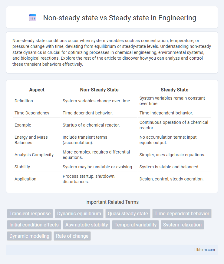
| Aspect | Non-Steady State | Steady State |
|---|---|---|
| Definition | System variables change over time. | System variables remain constant over time. |
| Time Dependency | Time-dependent behavior. | Time-independent behavior. |
| Example | Startup of a chemical reactor. | Continuous operation of a chemical reactor. |
| Energy and Mass Balances | Include transient terms (accumulation). | No accumulation terms; input equals output. |
| Analysis Complexity | More complex, requires differential equations. | Simpler, uses algebraic equations. |
| Stability | System may be unstable or evolving. | System is stable and balanced. |
| Application | Process startup, shutdown, disturbances. | Design, control, steady operation. |
Introduction to Non-Steady State and Steady State
Non-steady state refers to a dynamic condition where system variables such as concentration, temperature, or pressure change over time, reflecting transient behaviors. Steady state occurs when these variables remain constant despite ongoing processes, indicating equilibrium between inputs and outputs. Understanding the distinction between non-steady and steady states is crucial in fields like chemical engineering and biology for modeling reaction kinetics and system stability.
Defining Steady State: Key Characteristics
Steady state is characterized by constant system variables over time, where input and output rates are balanced, resulting in no net change in concentration, temperature, or other relevant parameters. Key characteristics include equilibrium conditions that ensure system stability and predictability, with mass and energy flows maintaining consistent levels. This contrasts with non-steady state scenarios, where variables fluctuate dynamically due to imbalanced inputs and outputs.
Understanding Non-Steady State Systems
Non-steady state systems involve dynamic processes where variables such as temperature, concentration, or pressure change over time, preventing equilibrium conditions. These systems are characterized by transient behaviors that require time-dependent analysis using differential equations to predict system responses accurately. Understanding non-steady state conditions is crucial for designing and optimizing processes like chemical reactors, thermal systems, and environmental modeling.
Fundamental Differences Between Steady State and Non-Steady State
Steady state refers to a condition where system variables remain constant over time despite ongoing processes, characterized by zero net change in mass, energy, or momentum within the system. Non-steady state occurs when these variables change dynamically over time due to transient conditions, leading to temporal variations in system behavior. The fundamental difference lies in the presence of time-dependent changes in non-steady state systems, whereas steady state systems exhibit time-invariant conditions.
Real-World Examples of Steady State Processes
Steady state processes maintain constant properties over time despite ongoing inputs and outputs, exemplified by the continuous operation of a power plant where energy input from fuel matches output electricity and heat dissipation. In chemical reactors running at steady state, reactant concentrations and temperature remain stable, enabling predictable product quality and efficient resource use. Similarly, in ecological systems like a mature forest, biomass and nutrient cycles reach a dynamic equilibrium, sustaining consistent ecosystem functions despite environmental fluctuations.
Non-Steady State Applications in Industry
Non-steady state processes, characterized by time-dependent changes in system variables, are crucial in industries requiring dynamic response adjustments such as batch chemical reactors, startup and shutdown operations, and transient heat exchangers. Industrial applications leverage non-steady state analysis for optimizing reaction times, improving safety during process transitions, and enhancing control strategies in processes where steady state conditions are not achievable. Understanding non-steady state behavior enables engineers to predict system responses, design efficient control systems, and minimize downtime in industries like pharmaceuticals, petrochemicals, and food processing.
Mathematical Representation of Both States
Non-steady state systems are characterized by variables that change with time, often represented by differential equations involving time derivatives, such as \(\frac{dC}{dt} = r(C,t)\), where \(C\) is the concentration and \(r\) a rate function. Steady state assumes that system variables remain constant over time, leading to algebraic equations obtained by setting time derivatives to zero, for example, \(\frac{dC}{dt} = 0\). The mathematical distinction hinges on solving time-dependent differential equations for non-steady states versus solving time-independent equations for steady states.
Impact on System Performance and Stability
Steady state conditions ensure system variables remain constant over time, promoting predictable performance and enhanced stability, which is critical for reliable operation in engineering systems. Non-steady state introduces transient behavior where system parameters fluctuate, potentially causing instability, performance degradation, and increased sensitivity to disturbances. Understanding the transition between non-steady and steady states enables optimization of control strategies to maintain system robustness and efficiency under dynamic conditions.
Importance in Engineering and Scientific Studies
Steady state conditions enable engineers and scientists to analyze systems with constant variables, simplifying mathematical modeling and ensuring predictable performance in process design. Non-steady state analysis captures dynamic behaviors and transient phenomena, crucial for understanding system responses to changes, start-up conditions, or disturbances. Mastery of both states enhances accuracy in simulation, control system design, and optimization of engineering processes such as chemical reactors, thermal systems, and fluid dynamics.
Choosing the Appropriate Model for Analysis
Choosing the appropriate model for analysis depends on whether the system behavior is constant or variable over time. Steady state models are ideal for systems with stable inputs and outputs, allowing simplification by assuming equilibrium conditions. Non-steady state models are essential when capturing transient behaviors, time-dependent changes, or dynamic responses to varying conditions.
Non-steady state Infographic