Stationary objects remain fixed in one position without any movement, playing a crucial role in various scientific and everyday contexts. Understanding the characteristics and applications of stationary states can enhance your grasp of physics, engineering, and even art. Explore the rest of the article to uncover the significance and nuances of stationary phenomena.
Table of Comparison
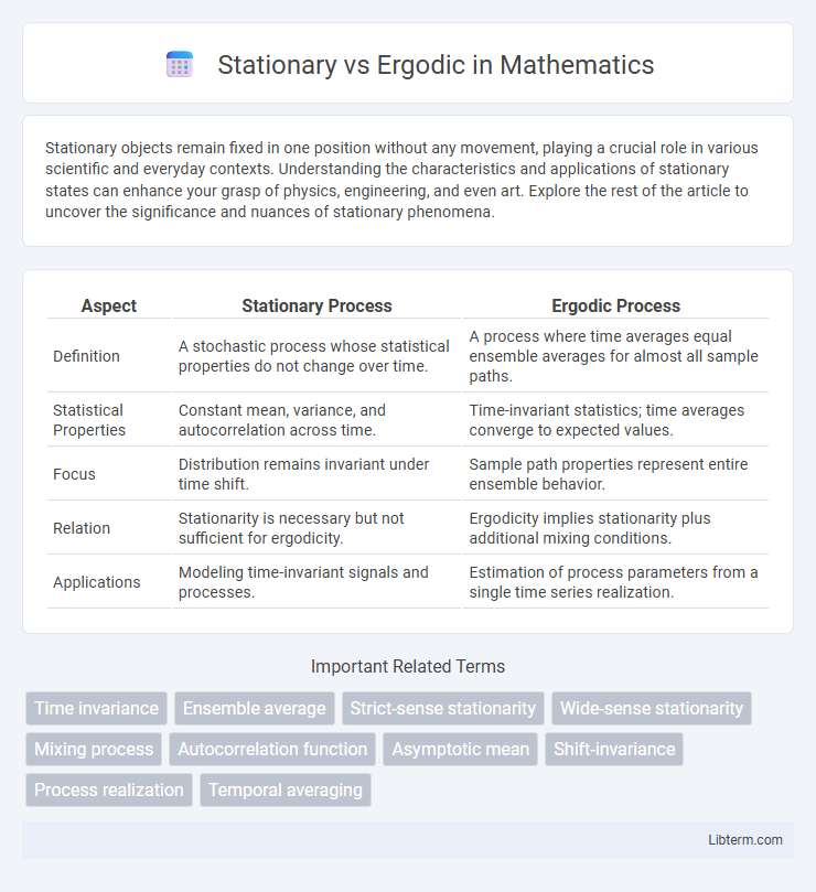
| Aspect | Stationary Process | Ergodic Process |
|---|---|---|
| Definition | A stochastic process whose statistical properties do not change over time. | A process where time averages equal ensemble averages for almost all sample paths. |
| Statistical Properties | Constant mean, variance, and autocorrelation across time. | Time-invariant statistics; time averages converge to expected values. |
| Focus | Distribution remains invariant under time shift. | Sample path properties represent entire ensemble behavior. |
| Relation | Stationarity is necessary but not sufficient for ergodicity. | Ergodicity implies stationarity plus additional mixing conditions. |
| Applications | Modeling time-invariant signals and processes. | Estimation of process parameters from a single time series realization. |
Introduction to Stationary and Ergodic Processes
Stationary processes exhibit statistical properties, such as mean and variance, that are constant over time, making them predictable in the context of time series analysis. Ergodic processes, a subset of stationary processes, allow time averages to equal ensemble averages, enabling meaningful long-term predictions from a single realization of the process. Understanding the distinction between stationary and ergodic processes is crucial for applying proper models in signal processing and stochastic analysis.
Defining Stationarity: Key Concepts
Stationarity in time series refers to a stochastic process whose statistical properties, such as mean, variance, and autocorrelation, remain constant over time. Strict stationarity requires the joint distribution of any set of variables to be invariant under time shifts, whereas weak stationarity only demands constant mean and autocovariance structure. Understanding these conditions is fundamental to distinguishing stationary processes from ergodic ones, where long-term averages converge to ensemble averages.
Understanding Ergodicity: Fundamental Principles
Ergodicity refers to a process where time averages and ensemble averages converge, ensuring long-term statistical properties can be deduced from a single trajectory. Unlike stationary processes, which maintain constant statistical characteristics over time, ergodic processes guarantee that sample paths represent the entire distribution. This fundamental principle is crucial in fields like thermodynamics, signal processing, and statistical mechanics for reliable inference and modeling.
Types of Stationarity in Time Series
Types of stationarity in time series include strict stationarity and weak stationarity, where strict stationarity requires the entire distribution of the series to be invariant over time, and weak stationarity requires only constant mean, variance, and autocovariance that depends solely on lag. Ergodicity, often linked with weak stationarity, implies that time averages converge to ensemble averages, enabling statistical properties to be inferred from a single time series realization. Understanding these types helps in selecting appropriate models such as ARMA or ARIMA for forecasting and in validating assumptions underlying statistical inference.
Ergodicity vs Stationarity: Core Differences
Ergodicity and stationarity are fundamental concepts in time series analysis, where stationarity implies that statistical properties such as mean and variance remain constant over time, while ergodicity ensures that time averages converge to ensemble averages, allowing a single time series realization to represent the entire process. A stationary process can be non-ergodic if its time averages do not reflect overall statistical behavior, whereas an ergodic process must be stationary to guarantee consistent inference from a single series. Understanding these distinctions is crucial for modeling stochastic processes and making valid predictions in fields like signal processing, economics, and meteorology.
Real-World Examples of Stationary Processes
Stationary processes maintain consistent statistical properties, such as mean and variance, over time, exemplified by daily temperature readings and certain financial time series like asset returns. Ergodic processes allow time averages to represent ensemble averages, enabling reliable long-term predictions from a single data sequence. Real-world stationary examples include white noise signals in electronics and steady-state signals in control systems, where probabilistic behavior remains stable across observations.
Practical Applications of Ergodic Processes
Ergodic processes are crucial in signal processing and communications, enabling reliable long-term statistical analysis from single time series data. Practical applications include network traffic modeling, where ergodicity ensures that time averages represent ensemble averages for system optimization. In wireless communications, ergodic assumptions facilitate performance evaluation of fading channels, improving resource allocation and system design.
Testing for Stationarity and Ergodicity
Testing for stationarity involves methods like the Augmented Dickey-Fuller (ADF) test and the KPSS test, which assess whether time series data have constant mean and variance over time. Ergodicity testing focuses on verifying if time averages converge to ensemble averages, often requiring analysis of autocorrelation functions or specialized hypothesis tests such as the Gikhman-Khasminskii criterion. Accurate diagnosis of stationarity and ergodicity is crucial for modeling and forecasting time series data reliably.
Importance in Data Science and Signal Processing
Stationary processes maintain consistent statistical properties over time, simplifying modeling and prediction in data science and signal processing by enabling reliable inference. Ergodic processes ensure time averages converge to ensemble averages, allowing single realizations to represent overall system behavior, which is critical for practical data analysis. Understanding the distinction enhances the accuracy of time series forecasting, noise reduction, and system identification in real-world applications.
Conclusion: Choosing Between Stationary and Ergodic Models
Choosing between stationary and ergodic models depends on the underlying data properties and the analysis goals. Stationary models assume constant statistical properties over time, making them suitable for time series with fixed means and variances, while ergodic models require time averages to represent ensemble averages, allowing for inference from single realizations when the process is ergodic. Understanding the data's temporal stability and whether ensemble characteristics can be inferred from time observations guides the optimal model selection for accurate predictions and insights.
Stationary Infographic