The Binomial Options Pricing Model provides a versatile framework for valuing options by simulating possible price movements over discrete time intervals. This model captures the probabilistic nature of market behavior, allowing for flexible assumptions about volatility and interest rates to estimate option premiums accurately. Discover how this method can enhance your option trading strategies by exploring the detailed mechanics in the rest of the article.
Table of Comparison
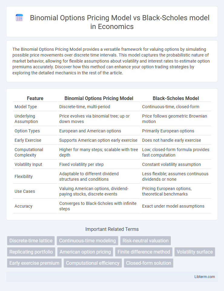
| Feature | Binomial Options Pricing Model | Black-Scholes Model |
|---|---|---|
| Model Type | Discrete-time, multi-period | Continuous-time, closed-form |
| Underlying Assumption | Price evolves via binomial tree; up or down moves | Price follows geometric Brownian motion |
| Option Types | European and American options | Primarily European options |
| Early Exercise | Supports American option early exercise | Does not handle early exercise |
| Computational Complexity | Higher for many steps; scalable with tree depth | Low; closed-form formula provides fast computation |
| Volatility Input | Fixed volatility per step | Constant volatility assumption |
| Flexibility | Adaptable to different dividend structures and conditions | Less flexible; assumes continuous dividends or none |
| Use Cases | Valuing American options, dividend-paying stocks, discrete events | Pricing European options, theoretical benchmarks |
| Accuracy | Converges to Black-Scholes with infinite steps | Exact under model assumptions |
Introduction to Options Pricing Models
The Binomial Options Pricing Model uses a discrete-time framework to estimate option prices by simulating multiple possible price paths of the underlying asset, accommodating American options and early exercise features. The Black-Scholes model provides a continuous-time closed-form solution, primarily applied to European options, relying on assumptions like constant volatility and risk-free interest rates. Both models are foundational in financial derivatives pricing, with the binomial model offering flexibility and the Black-Scholes model delivering analytical elegance.
Overview of the Binomial Options Pricing Model
The Binomial Options Pricing Model uses a discrete-time framework to evaluate options by simulating multiple possible price paths of the underlying asset over the option's life. This model constructs a binomial price tree, where at each node the asset price can move up or down by specific factors, allowing flexible incorporation of varying conditions like dividends or American-style exercise features. Its step-by-step backward induction process calculates option values at expiration and traces them back to the present, making it highly adaptable for complex option valuation compared to the continuous-time Black-Scholes model.
Fundamentals of the Black-Scholes Model
The Black-Scholes model fundamentally relies on the assumption of continuous-time stochastic processes and geometric Brownian motion for underlying asset prices, enabling closed-form solutions for European option pricing. Key parameters include volatility, risk-free interest rate, time to maturity, and strike price, which collectively determine the option's theoretical price through partial differential equations. This model contrasts with the Binomial Options Pricing Model by offering computational efficiency and analytical precision, while assuming constant volatility and log-normal distribution of asset returns.
Key Mathematical Assumptions Compared
The Binomial Options Pricing Model assumes a discrete-time framework where the underlying asset price can move to two possible values at each step, enabling flexible modeling of American-style options with early exercise features. The Black-Scholes model relies on continuous-time assumptions, modeling asset prices as a geometric Brownian motion with constant volatility and risk-free rate, suitable primarily for European options. Both models assume no arbitrage, frictionless markets, and log-normal distribution of asset prices but differ fundamentally in their approach to time and exercise rights.
Model Flexibility and Practical Applications
The Binomial Options Pricing Model offers greater flexibility by accommodating varying exercise opportunities and changing volatility, making it suitable for American options and complex derivatives with multiple decision points. In contrast, the Black-Scholes model provides a closed-form analytical solution optimized for European options with continuous trading assumptions, offering computational efficiency but limited adaptability to real-world conditions like early exercise or discrete dividends. Practical applications favor the Binomial model for scenarios requiring step-by-step exercise decisions, while the Black-Scholes model remains widely used for pricing standard European options under stable market assumptions.
Handling American vs. European Options
The Binomial Options Pricing Model excels in valuing American options by allowing for early exercise at each node in its discrete time framework, whereas the Black-Scholes model is primarily designed for European options with exercise only at maturity. This makes the Binomial model more versatile for American options, capturing optimal exercise strategies through a step-by-step lattice approach. The Black-Scholes formula relies on continuous-time assumptions and closed-form solutions, limiting its direct applicability to American options without modifications or approximations.
Accuracy in Volatile and Complex Markets
The Binomial Options Pricing Model offers greater accuracy in volatile and complex markets by accommodating varying conditions over multiple time steps, allowing dynamic adjustments to underlying asset prices and volatility. In contrast, the Black-Scholes model assumes constant volatility and lognormal distribution of asset returns, which can lead to inaccuracies during rapid market fluctuations or when dealing with American-style options. Therefore, the Binomial model is often preferred for pricing options in markets with high uncertainty and complex features, while Black-Scholes remains a faster, more streamlined approach for stable environments.
Computational Complexity and Efficiency
The Binomial Options Pricing Model involves iterative calculations across multiple time steps, resulting in higher computational complexity especially for large time grids, yet it offers flexibility for American options and various payoff structures. In contrast, the Black-Scholes model relies on closed-form analytical solutions, providing significantly faster computation and efficiency but is limited to European-style options with constant volatility assumptions. The trade-off between model flexibility and computational efficiency often guides the choice depending on the option type and required precision.
Advantages and Limitations of Each Model
The Binomial Options Pricing Model offers flexibility in handling American options and allowing for changing volatility and dividends over time, making it suitable for complex option features, but it can be computationally intensive with increased time steps. The Black-Scholes model provides closed-form analytical solutions for European options with constant volatility and no dividends, enabling faster calculations, yet it struggles with American options and assumptions of constant volatility limit its accuracy in real markets. Each model's strengths and weaknesses depend on the option type and market conditions, requiring careful selection based on the specific pricing scenario.
Choosing the Right Model for Option Valuation
Binomial Options Pricing Model offers flexibility for valuing American options due to its ability to model early exercise features, while the Black-Scholes model is preferred for European options with continuous trading assumptions. The binomial model's discrete-time lattice approach accommodates changing volatility and varying dividends, making it suitable for complex scenarios. In contrast, Black-Scholes provides faster computation and analytical solutions, ideal for straightforward, constant-parameter environments.
Binomial Options Pricing Model Infographic