The Linear Probability Model (LPM) is a simple regression approach used to estimate binary outcome variables by modeling the probability of an event occurring as a linear function of predictor variables. Despite its ease of interpretation, the model may produce predicted probabilities outside the 0-1 range and assumes constant variance, which can lead to inefficiencies. Explore the rest of this article to understand the advantages, limitations, and practical applications of the Linear Probability Model in your analyses.
Table of Comparison
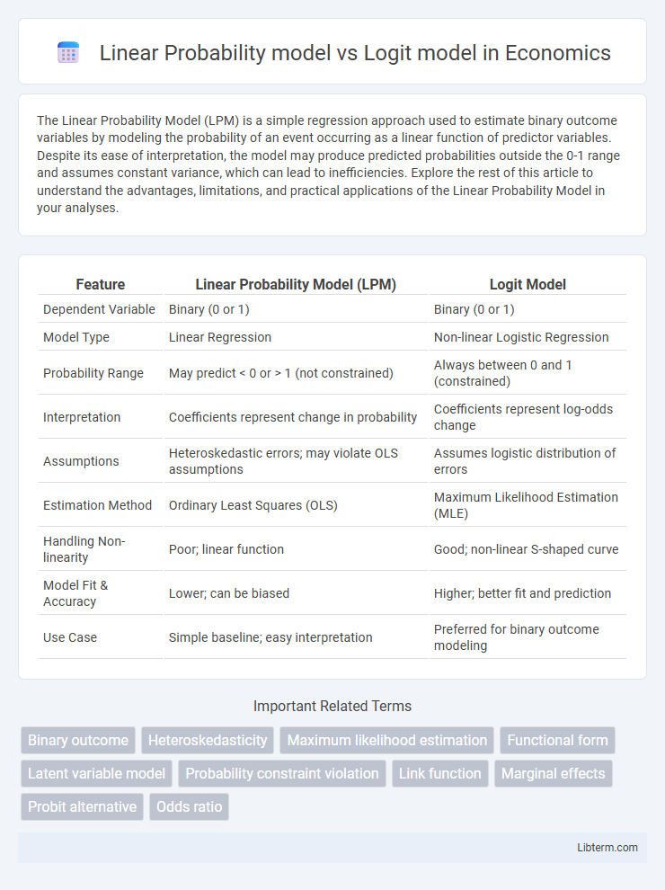
| Feature | Linear Probability Model (LPM) | Logit Model |
|---|---|---|
| Dependent Variable | Binary (0 or 1) | Binary (0 or 1) |
| Model Type | Linear Regression | Non-linear Logistic Regression |
| Probability Range | May predict < 0 or > 1 (not constrained) | Always between 0 and 1 (constrained) |
| Interpretation | Coefficients represent change in probability | Coefficients represent log-odds change |
| Assumptions | Heteroskedastic errors; may violate OLS assumptions | Assumes logistic distribution of errors |
| Estimation Method | Ordinary Least Squares (OLS) | Maximum Likelihood Estimation (MLE) |
| Handling Non-linearity | Poor; linear function | Good; non-linear S-shaped curve |
| Model Fit & Accuracy | Lower; can be biased | Higher; better fit and prediction |
| Use Case | Simple baseline; easy interpretation | Preferred for binary outcome modeling |
Introduction to Linear Probability and Logit Models
The Linear Probability Model (LPM) estimates binary outcomes using a linear regression framework, providing simplicity but often producing predicted probabilities outside the [0,1] range. The Logit model addresses this limitation by employing a logistic function to model the probability, ensuring outputs remain between 0 and 1 and capturing nonlinear relationships between predictors and the binary dependent variable. Both models are fundamental in binary response analysis, with the Logit model offering greater statistical rigor and interpretability for classification tasks.
Understanding Binary Outcome Modeling
The Linear Probability Model (LPM) uses a simple linear regression framework to estimate the probability of a binary outcome, treating the dependent variable as continuous, which can lead to predicted probabilities outside the 0-1 range and heteroscedasticity issues. The Logit model applies a logistic function to ensure predicted probabilities lie strictly between 0 and 1, making it more appropriate for binary outcome modeling by accounting for the non-linear relationship between predictors and the event probability. Logit also provides interpretable odds ratios and better handles non-constant variance, improving the robustness and accuracy of binary classification tasks.
The Linear Probability Model: Definition and Formulation
The Linear Probability Model (LPM) is a regression approach used to estimate binary outcome variables, where the dependent variable takes values of 0 or 1. It formulates the probability of an event occurring as a linear function of predictor variables, expressed as P(Y=1|X) = Xb + e, where b represents the coefficient vector and e is the error term. Despite its simplicity and ease of interpretation, the LPM can produce predicted probabilities outside the [0,1] range, which limits its practical applicability in modeling binary response data.
Key Features and Assumptions of the Linear Probability Model
The Linear Probability Model (LPM) uses ordinary least squares to estimate binary dependent variables, assuming a linear relationship between predictors and the probability of an event. Key features include ease of interpretation and computational simplicity, but the model often predicts probabilities outside the [0,1] range and assumes constant variance of errors, violating homoscedasticity. Unlike the Logit model, which relies on a logistic function to ensure predicted probabilities remain between 0 and 1 and accounts for non-linear relationships, the LPM's assumptions can lead to biased and inefficient estimates when applied to binary outcomes.
Introduction to the Logit Model
The Logit model estimates the probability of a binary outcome by modeling the log-odds as a linear function of predictors, ensuring predicted probabilities lie between 0 and 1. Unlike the Linear Probability Model (LPM), which can produce probabilities outside the feasible range and suffers from heteroscedasticity, the Logit model uses the logistic function to convert linear combinations into valid probabilities. This model provides consistent, efficient maximum likelihood estimates, making it preferable for binary response modeling in econometrics and statistics.
Core Characteristics and Theoretical Basis of Logit Model
The Linear Probability Model (LPM) predicts binary outcomes using a linear regression framework but often yields predicted probabilities outside the 0-1 range, leading to interpretation challenges. In contrast, the Logit Model is grounded in logistic regression theory, modeling the log-odds of the dependent variable as a linear combination of predictors, ensuring predicted probabilities remain strictly between 0 and 1. The Logit Model's theoretical foundation in the logistic distribution provides a nonlinear, S-shaped curve that better captures probability behavior in classification tasks and resolves heteroscedasticity issues inherent in LPM.
Comparison: Interpretation of Coefficients
The Linear Probability Model (LPM) coefficients represent the change in the probability of the dependent binary outcome for a one-unit change in the predictor, offering direct interpretability but often leading to predicted probabilities outside the [0,1] range. In contrast, Logit model coefficients reflect changes in the log-odds of the dependent variable occurring, necessitating transformation via the logistic function to obtain predicted probabilities, which always remain between 0 and 1. This makes the Logit model more suitable for binary response variables, providing a nonlinear relationship that respects probability boundaries and allowing for odds ratio interpretation.
Practical Differences: Prediction and Probability Bounds
The Linear Probability Model (LPM) directly estimates probabilities but often produces predicted values outside the [0,1] range, leading to interpretability issues. The Logit model uses a logistic function to constrain predicted probabilities strictly between 0 and 1, ensuring more realistic and reliable estimates. In practice, Logit models provide better probability bounds and handle binary outcome prediction with higher accuracy compared to the LPM.
Advantages and Limitations: Linear Probability vs Logit Model
The Linear Probability Model (LPM) offers simplicity and ease of interpretation through its direct estimation of probabilities using linear regression, but it suffers from heteroscedasticity and can predict probabilities outside the [0,1] range. The Logit model, employing a logistic function, ensures predicted probabilities remain within logical bounds and accounts for non-linearity, providing better fit and interpretation for binary outcomes. However, the Logit model's complexity requires iterative estimation methods and may be less intuitive for direct coefficient interpretation compared to the LPM.
Choosing the Right Model for Binary Outcomes
Choosing the right model for binary outcomes depends on the relationship between predictors and the probability of the event. The Linear Probability Model (LPM) offers simplicity and ease of interpretation by estimating probabilities directly but suffers from heteroscedasticity and predictions outside the [0,1] range. Logit models address these issues by using a logistic function to constrain predicted probabilities within the unit interval and accommodate non-linear relationships, making them more appropriate for binary dependent variables with complex predictor interactions.
Linear Probability model Infographic