The binomial theorem simplifies the process of expanding expressions raised to a power, such as (a + b)^n, by providing a clear formula involving binomial coefficients. Understanding binomial distributions is essential in statistics for modeling the number of successes in a fixed number of independent trials. Explore the rest of this article to deepen your understanding of binomial concepts and their practical applications.
Table of Comparison
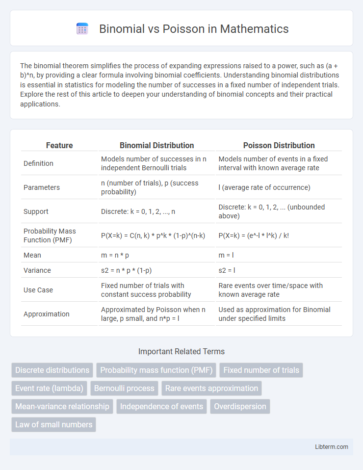
| Feature | Binomial Distribution | Poisson Distribution |
|---|---|---|
| Definition | Models number of successes in n independent Bernoulli trials | Models number of events in a fixed interval with known average rate |
| Parameters | n (number of trials), p (success probability) | l (average rate of occurrence) |
| Support | Discrete: k = 0, 1, 2, ..., n | Discrete: k = 0, 1, 2, ... (unbounded above) |
| Probability Mass Function (PMF) | P(X=k) = C(n, k) * p^k * (1-p)^(n-k) | P(X=k) = (e^-l * l^k) / k! |
| Mean | m = n * p | m = l |
| Variance | s2 = n * p * (1-p) | s2 = l |
| Use Case | Fixed number of trials with constant success probability | Rare events over time/space with known average rate |
| Approximation | Approximated by Poisson when n large, p small, and n*p = l | Used as approximation for Binomial under specified limits |
Introduction to Binomial and Poisson Distributions
Binomial and Poisson distributions are fundamental probability distributions used in statistics to model discrete random variables. The binomial distribution applies to scenarios with a fixed number of independent trials, each with the same probability of success, and is characterized by parameters n (number of trials) and p (probability of success). The Poisson distribution models the number of events occurring in a fixed interval of time or space when these events happen with a known constant mean rate and independently of the time since the last event, with parameter l (the average rate of occurrence).
Key Differences Between Binomial and Poisson
The key differences between Binomial and Poisson distributions lie in their parameters and applications: the Binomial distribution is defined by the number of trials (n) and probability of success (p), used for fixed number of independent experiments with two possible outcomes. The Poisson distribution is characterized by the mean number of occurrences (l) in a fixed interval, modeling rare events occurring independently over time or space. Binomial is discrete with a fixed number of trials, while Poisson assumes an unlimited number of potential occurrences and is often used as an approximation of the Binomial when n is large and p is small.
Definitions and Basic Concepts
The binomial distribution models the number of successes in a fixed number of independent trials, each with the same probability of success. The Poisson distribution describes the probability of a given number of events occurring in a fixed interval of time or space, assuming events happen independently at a constant average rate. Both distributions are discrete, but binomial requires a fixed number of trials while Poisson is used for events with potentially unlimited occurrences.
Mathematical Formulations
The Binomial distribution is defined by the probability mass function P(X = k) = C(n, k) p^k (1 - p)^(n - k), where n is the number of trials, p is the probability of success, and k is the number of successes. The Poisson distribution is defined by P(X = k) = (l^k e^{-l}) / k!, where l represents the average rate of occurrence within a fixed interval and k is the count of occurrences. The Poisson distribution emerges as a limiting case of the Binomial distribution when n approaches infinity and p approaches zero while the product n*p remains constant at l.
Assumptions and Conditions of Each Model
The Binomial distribution assumes a fixed number of independent trials with only two possible outcomes (success or failure) and a constant probability of success in each trial. The Poisson distribution models the number of events occurring in a fixed interval of time or space, assuming events happen independently and at a constant average rate. While the Binomial applies when the number of trials is known and probability is fixed, the Poisson is suitable for modeling rare events with a potentially infinite number of occurrences.
Real-World Applications: Binomial vs Poisson
The Binomial distribution models the number of successes in a fixed number of independent trials with a constant probability of success, making it ideal for quality control processes and clinical trial outcomes. The Poisson distribution describes the number of events occurring in a fixed interval of time or space when events happen independently at a constant rate, which suits applications like modeling call arrivals in call centers or traffic flow analysis. Understanding the distinct scenarios for Binomial and Poisson helps optimize decision-making in fields such as manufacturing, telecommunications, and epidemiology.
When to Use Binomial Distribution
The binomial distribution is ideal when modeling the number of successes in a fixed number of independent trials, each with the same probability of success. Use the binomial distribution when the total number of trials (n) and the probability of success (p) are known and the outcomes are binary, such as pass/fail or yes/no. This contrasts with the Poisson distribution, which is better suited for modeling the count of events occurring within a fixed interval when the event rate is low and the number of trials is large or unknown.
When to Use Poisson Distribution
The Poisson distribution is ideal for modeling the number of rare events occurring within a fixed interval of time or space when the average rate is known and events occur independently. Use Poisson when the number of trials is large, the probability of success is small, and the binomial distribution becomes cumbersome to calculate. Typical applications include counting arrivals at a service point, radioactive decay events, or the occurrence of defects in manufacturing processes.
Example Problems and Solutions
Binomial distribution models the number of successes in a fixed number of independent trials with a constant probability, such as calculating the probability of getting exactly 3 heads in 5 coin tosses. Poisson distribution predicts the number of events occurring within a fixed interval, typically used for rare events like the probability of 4 customer arrivals in an hour at a bank. Example solutions involve using the binomial probability formula P(X=k) = C(n,k)p^k(1-p)^(n-k) for discrete trials, while Poisson probability is calculated by P(X=k) = (l^k e^-l)/k! for event counts over time or space.
Summary: Choosing the Right Distribution
The Binomial distribution is ideal for modeling the number of successes in a fixed number of independent trials with a constant probability of success, typically used when the number of trials n and probability p are known and outcomes are binary. The Poisson distribution is better suited for modeling the count of events occurring in a fixed interval of time or space when events happen independently with a known constant mean rate l, especially useful when n is large and p is small in Binomial scenarios. Choosing the right distribution depends on the experiment setup: use the Binomial when trials are fixed and success probability is constant, and the Poisson when events are rare and occur independently over time or space.
Binomial Infographic